Solving Initial Value Problems Numerically in Python with SciPy

Jul 4, 2022

Using SciPy's solve_ivp to solve initial value problems

Edits:

Apr 16, 2023 : Changing image and file paths
Oct 12, 2023 : Changing picture and file paths

Introduction

In this post, we’ll look at how we can use the solve_ivp function from scipy.integrate in order to solve ordinary differential equations with initial values numerically.

A Simple One-Variable Problem

To start with, we’re going to start with a simple, one-variable system whose answer we can solve for exactly in order to verify that the numerical solver works in the way that we expect. The well-known ODE for exponential growth:

\frac{d}{dt}f(t) = f(t),\ f(0) = f_0

This can be solved exactly, and gives the solution $f(t) = f_0 e^t$ . Now let’s see how we can solve this using solve_ivp from scipy.integrate. This function has the signature solve_ivp(func, times, y_0, ...), where of course there many other options.

Here, the callable func itself represents the system of ODEs, and has the signature func(t, y), where $t$ is the one-dimensional variable on which the system depends and $y$ is a vector representing the current state of the system. The returned value should be the vector of derivatives at time $t$ and state $y$ . More mathematically, we want func such that

\frac{d\vec{y}}{dt} = func(t, \vec{y})

The parameter times is a tuple (start, stop) of times to integrate the system over. The system will begin at time start and end at time stop. The parameter y_0 is the initial state of the system at time start.

For our simple system then, we can solve the system over the interval $t\in [ 0, 5 ]$ with initial value $f(0) = 1$ as follows:

from scipy.integrate import solve_ivp
import numpy as np
import matplotlib.pyplot as plt

def func(t, state):
    """ Returns the derivative at the given time and state """
    return state

times = (0, 5)
initial_value = [1]

results = solve_ivp(func, times, initial_value)

# Now let's plot the results against the actual solution
fig, ax = plt.subplots()
fig.suptitle(f"Solution to df/dt = f(t), f(0) = 1")
ax.set_xlabel('t')
ax.set_ylabel('f(t)')
ax.plot(results.t, results.y[0], label="Solved Numerically") # numerically
ts = np.linspace(*times, 100)
ax.plot(ts, np.exp(ts), label="Exact Solution") # exact
fig.legend()

plt.savefig('1dsystem.png')

The final result is

  message: 'The solver successfully reached the end of the integration interval.'
     nfev: 32
     njev: 0
      nlu: 0
      sol: None
   status: 0
  success: True
        t: array([0.        , 0.10001999, 1.06609106, 2.30431769, 3.64528981,
       5.        ])
 t_events: None
        y: array([[  1.        ,   1.10519301,   2.9040598 ,  10.01740317,
         38.29174533, 148.39440874]])
 y_events: None

We can see that there is a lot of additional information passed back, in addition to the numerical values of the function at the given times! For our purposes, there are a few attributes of the returned object which are particulary important.

results.t is an array of the times $t$ at which the system was evaluated.
results.y is an array of arrays, each of which corresponds to the state of the system at one particular time $t$ . The array represents the system in the same way as the $y$ parameter to the callable func which you passed into solve_ivp.

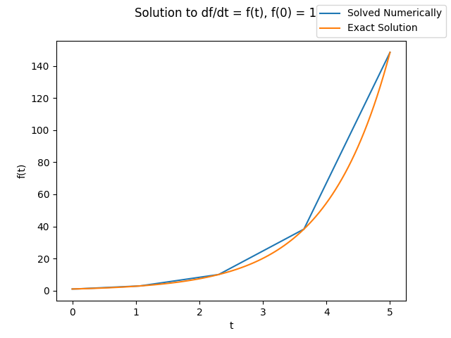
However, just by staring at this it is not at all obvious that it is actually correct. Let’s quickly plot this against the actual solution:

Numerical and exact solutions to df/dt = f(t), f(0) = 1

from scipy.integrate import solve_ivp
import numpy as np
import matplotlib.pyplot as plt

def func(t, state):
    """ Returns the derivative at the given time and state """
    return state

times = (0, 5)
initial_value = [1]

results = solve_ivp(func, times, initial_value)

# Now let's plot the results against the actual solution
fig, ax = plt.subplots()
fig.suptitle(f"Solution to df/dt = f(t), f(0) = 1")
ax.set_xlabel('t')
ax.set_ylabel('f(t)')
ax.plot(results.t, results.y[0], label="Solved Numerically") # numerically
ts = np.linspace(*times, 100)
ax.plot(ts, np.exp(ts), label="Exact Solution") # exact
fig.legend()

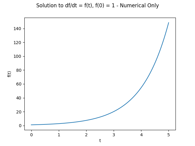
plt.savefig('1dsystem.png')

From the graph, we can see that the agreement seems to be good. One oddity is that the numerical solution is only defined for five points over the interval, and by looking at the actual values of results.t they are not evenly spaced or anything like that. In fact, those particular points are automatically selected by solve_ivp in order to keep the accumulated error between the exact and numerical solutions below a certain threshold. However, we can control this in a variety of ways. The easiest is probably to set the max_step parameter, but another way would be to explicitly pass in a list of $t$ values at which to evaluate the system. I prefer the max_step option, since it leaves open the possibility that the step can be shorter for the case in which additional accurracy is needed when solving. To solve the system numerically and plot that solution with much shorter steps would look as follows:

Numerical Solution to df/dt = f(t), f(0) = 1

from scipy.integrate import solve_ivp
import numpy as np
import matplotlib.pyplot as plt

def func(t, state):
    """ Returns the derivative at the given time and state """
    return state

times = (0, 5)
initial_value = [1]

results = solve_ivp(func, times, initial_value, max_step=0.01)

fig, ax = plt.subplots()
fig.suptitle(f"Solution to df/dt = f(t), f(0) = 1 - Numerical Only")
ax.set_xlabel('t')
ax.set_ylabel('f(t)')
ax.plot(results.t, results.y[0], label="Solved Numerically") # numerically
plt.savefig('1dsystem-numerical.png')

Again, just by looking we can see that the solution looks as we expect.

Two Variables: Lotka-Volterra System

Now let’s look at another, slightly more complex system. The Lotka-Volterra model of predator-prey interaction is given by the following:

\begin{align*} \frac{dx}{dt} &= x(b - py) \\ \frac{dy}{dt} &= y(rx - d) \\ \end{align*}

Where

$x$ is the population of the prey species
$y$ is the population of the predator species

And the parameter

$b$ represents the growth rate of the prey species in the absence of predation
$p$ has something to do with how often / likely it is that the predator species eats the prey species
$r$ has something to do with how much food each member of the prey species provides
$d$ is the death rate of the predator species

There are a few additional wrinkles to this problem. First of all, it now lives in three dimensions: time, prey population, and predator population. In addition, we have a bunch of additional parameters that we need to pass in to our function. Let’s see how we can solve each of these problems, and see a plot of the solution.

from scipy.integrate import solve_ivp
import numpy as np
import matplotlib.pyplot as plt

def func(t, state, b, p, r, d):
    x, y = state
    dxdt = x * (b - p * y)
    dydt = y * (r * x - d)
    return dxdt, dydt

times = 0, 15
y_0 = 0.5, 0.5

results = solve_ivp(func, times, y_0, args=(1, 1, 1, 1), max_step=0.01)

fig, ax = plt.subplots()
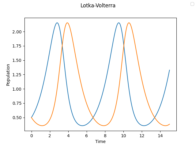
fig.suptitle("Lotka-Volterra")
ax.set_xlabel('Time')
ax.set_ylabel('Population')
fig.legend()
ax.plot(results.t, results.y[0], label="Prey Population")
ax.plot(results.t, results.y[1], label="Predator Population")
plt.savefig('lotkavolterra.png')

Numerical solution to the Lotka-Volterra System

A few things to note:

Since our state function now took additional variables, we needed to pass these as an arguments args=(...) to solve_ivp. Alternate solutions would be to hard-code these values into the function or to curry the function to remove these arguments, but I find that this way is the most explicit and easiest to understand.

Our solution now contains two quantities: $x$ and $y$ . These are stored in results.y[0] and results.y[1], respectively. If we wanted, we could plot the phase-space diagram of the system by plotting these agaist each other to verify the apparent periodicity of the solution, but for now let’s just take it on faith.

Three Variables: The Lorenz System

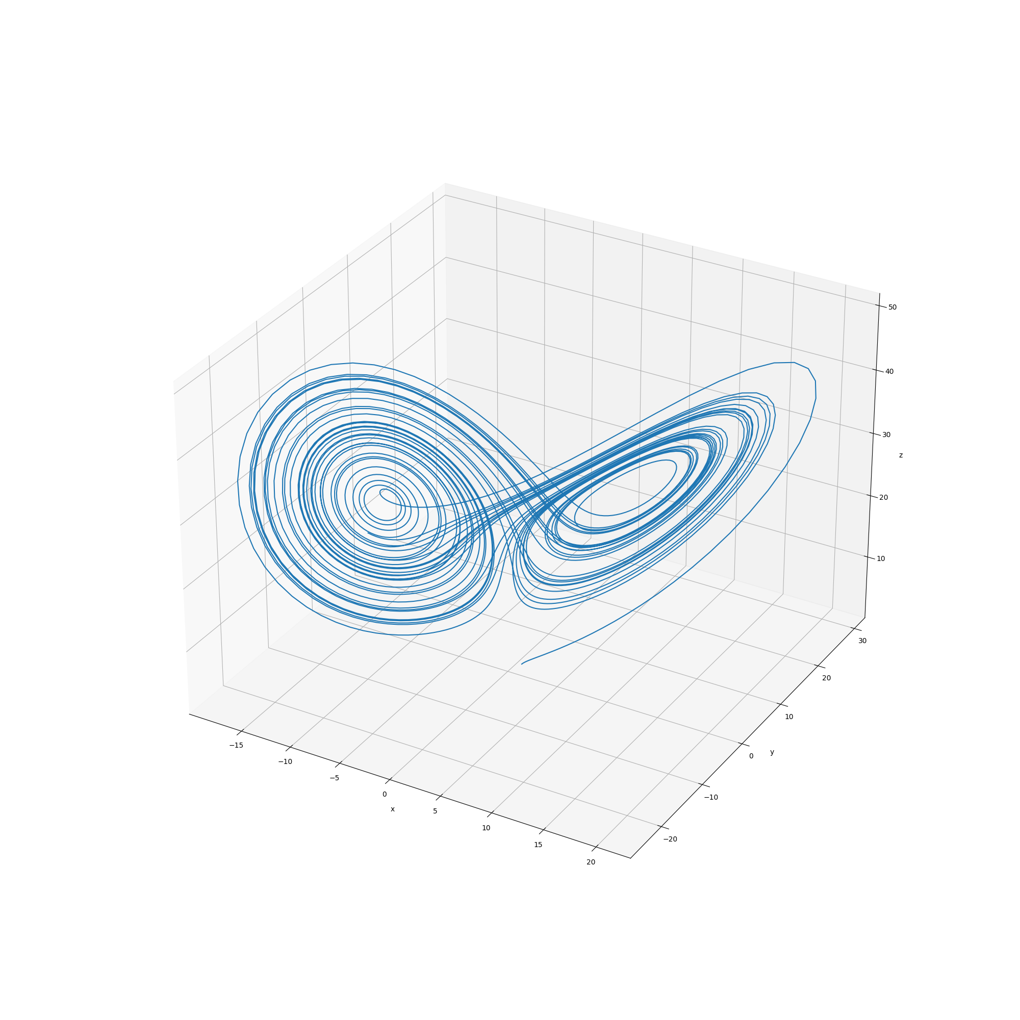
For fun, let’s take this a step further and take a look at the very famous 3-variable Lorenz system. This system is an extremely simplified model of the atmosphere, and is particularly notable because it was one of the first documented instances of chaotic behaviour. The system itself is given by

\begin{align*} \frac{dx}{dt} &= \sigma(y - x) \\ \frac{dy}{dt} &= x(\rho - z) - y \\ \frac{dz}{dt} &= xy - \beta z \\ \end{align*}

The values of the parameters originally used by Lorenz were $\sigma=10$ , $\beta=\frac{8}{3}$ , and $\rho = 28$ , for which the system exhibits choatic behaviour. Now let’s solve this numerically and plot the phase space diagram thereof!

from scipy.integrate import solve_ivp
import numpy as np
import matplotlib.pyplot as plt

def func(t, state, sigma, beta, rho):
    x, y, z = state
    dxdt = sigma * (y - x)
    dydt = x * (rho - z)
    dzdt = x * y - beta * z
    return dxdt, dydt, dzdt

y0 = 1, 1, 1
ts = 1, 40
results = solve_ivp(func, ts, y0, args=(10, 8/3, 28), max_step=0.01)

# plot the results as a phase-space diagram
fig = plt.figure(figsize=(20, 20))
ax = fig.gca(projection="3d")
ax.set_xlabel('x')
ax.set_ylabel('y')
ax.set_zlabel('z')
ax.plot(results.y[0], results.y[1], results.y[2])

plt.savefig('lorenz.png')

Phase space diagram of a numerical solution to the Lorenz system

Conclusion

We can use the solve_ivp function from scipy.integrate in order to quickly and easily solve initial value problems for systems of ordinary differential equations numerically. Of course, what we have done here is just scratching the surface - there are many more parameters that solve_ivp takes, and the documentation is very good.

Sources and Further Reading

The initial inspiration for this post: Differential Equations in Python with SciPy - Daniel Müller-Komorowska
Documentation for solve_ivp
Wikipedia (Lotka-Volterra)
Wikipedia (Lorenz system)