How Quickly Did Tyrannosaurs Grow? Curve Fitting with SciPy

Aug 1, 2022

How to use SciPy's curve_fit function to optimize function parameters

Edits:

Apr 15, 2022 : Changing picture and file paths
Oct 12, 2023 : Changing picture and file paths

Introduction

Lately, I’ve become more interested in paleontology and have started to read more and more scientific papers on the subject. I’ve also become more initerested in statistics, so to improve at both of these, have begun to try to recreate simple statistical analyses from the papers. In this article, I’m going to (attempt to) recreate the growth curve for Tyrannosaurus rex as found in (Ericson, et. al. 2004). To do so, I am going to need to fit a logistic curve to the data they collected, using SciPy’s curve_fit function!

An Example - Linear Regression

To begin with, let’s start with the simplest application of curve_fit: performing a linear regression. Let’s generate some fake data to start. The data itself will be of the form $y = 2x + 3 + \epsilon$ , with $\epsilon \sim N(0, 1)$ .

# Generate random data fitting a linear equation y = 2x + 3 + N(0, 1)

xs <- seq(-3, 3, 0.5)
sigma <- 1
errors <- rnorm(length(xs), 0, sigma)
ys <- 2 * xs + 3 + errors
data <- data.frame(x=xs, y=ys)
write.csv(data, "linear_data.csv", row.names=F)

png(file="linear_data.png")
	plot(ys ~ xs, main="Linear Data (with noise)", xlab="x", ylab="y")
	curve(2*x+3, add=T)
dev.off()

The data itself looks as follows:

"x","y"
-3,-2.85528637087481
-2.5,-0.2839377919616
-2,-0.862210829714574
-1.5,-0.637626631963547
-1,1.24584946456147
-0.5,1.31450035272819
0,2.14133679507907
0.5,6.61915638937528
1,5.14362896464176
1.5,5.63355382223453
2,7.19223928757166
2.5,7.36080742979852
3,7.87498175608272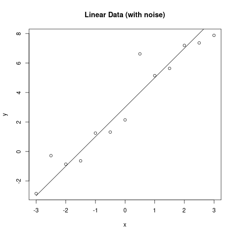

Initial Fake Linear Data

Now let’s fit the data! The general shape of the curve_fit function is curve_fit(f, xdata, ydata). Here, f is a callable (a function) which takes in an $x$ value as its first parameter and then the actual parameters to be fit as the others: f(x, *params). What curve_fit is attempting to do is find the parameters which minimize the least-squares distance between f(xdata, *params) and ydata. Nominally, we expect ydata = f(xdata, *params).

The return value for curve_fit is [popt, pcov], where popt are the optimal parameters and pcov is the variance-covariance matrix between the different parameters. For now, we will be mostly ignoring pcov.

So what does this look like for us? Well, we want to fit a linear function of the form $f(x) = mx + b$ , so we will have two parameters: $m$ and $b$ . Our function in Python will look like

def linear_curve(x, m, b):
	return m * x + b

The entire program to load in the data, find an optimal solution, and plot it are as follows:

import pandas as pd
import matplotlib.pyplot as plt

from scipy.optimize import curve_fit

def linear_curve(x, m, b) -> float:
    return m * x + b

df = pd.read_csv('./linear_data.csv')

result = curve_fit(linear_curve, df['x'], df['y'])
popt, pcov = result
m, b = popt

fig, ax = plt.subplots()
fig.suptitle('Fitting a Linear Curve')
ax.set_xlabel('x')
ax.set_ylabel('y')
ax.plot('x', 'y', 'ko', data=df, label="Raw Data")
ax.plot(df['x'], 2 * df['x'] + 3, 'k-', label="Actual")
ax.plot(df.x, m * df.x + b, 'r--', label=f"Fitted - m={m:.2f}, b={b:.2f}")
ax.legend()
fig.savefig('fitted_linear_curve.jpg')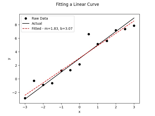

Linear Fit

We can see that we are getting a good agreement between the actual function used to generate the data and what we extracted using curve fitting.

Fitting a Logistic Curve

Now that we have an idea of how the function works, let’s take a look at what we actually want to do: fit a logistic curve to some Tyrannosaurus growth data! First, let’s take a look at the data.

Age (Years)	Mass (kg)
28	5654
22	5040
18	3230
16	2984
14	1807
15	1761
2	29.9

(Data from Erickson et at 2004 Table 1)

For our purposes, let’s fit this with a very general logistic curve:

f(x) = \frac{A}{1 + e^{-k(x-x_0)}} + E

So now we have four parameters instead of two, but apart from that the process is the same. So, let’s load in the data, fit the curve, and plot the results!

import numpy as np
import pandas as pd
import matplotlib.pyplot as plt

from scipy.optimize import curve_fit

def logistic(x, A, k, x_0, offset) -> float:
    expected = A / (1 + np.exp(-k * (x - x_0))) + offset
    return expected

df = pd.read_csv('./tyrannosaurus_growth_table.csv', dtype={'age': np.double, 'mass': np.double})
print(df)

popt, pcov = curve_fit(logistic, df.age, df.mass )
A, k, x_0, offset = popt

ages = np.linspace(0, 30, 101)
masses = logistic(ages, *popt)

fig, ax = plt.subplots()
fig.suptitle("Tyrannosaurus Rex Growth Curve")
ax.plot('age', 'mass', 'ko', data=df, label="Data")
ax.plot(ages, masses, 'k-', data=df, label="Fitted Curve")
ax.set_xlabel('Age (Years)')
ax.set_ylabel('Mass (kg)')
ax.legend()
fig.savefig("tyrannosaurus_growth_curve.jpg")

Disaster! If you try running this you get a very nasty looking error:

/home/eric/.local/lib/python3.8/site-packages/scipy/optimize/minpack.py:833: OptimizeWarning: Covariance of the parameters could not be estimated
  warnings.warn('Covariance of the parameters could not be estimated',
Traceback (most recent call last):
  File "fit_logistic.py", line 24, in <module>
    ax.plot(ages, masses, 'k-', data=df, label="Fitted Curve")
  File "/home/eric/.local/lib/python3.8/site-packages/matplotlib/axes/_axes.py", line 1605, in plot
    lines = [*self._get_lines(*args, data=data, **kwargs)]
  File "/home/eric/.local/lib/python3.8/site-packages/matplotlib/axes/_base.py", line 315, in __call__
    yield from self._plot_args(this, kwargs)
  File "/home/eric/.local/lib/python3.8/site-packages/matplotlib/axes/_base.py", line 501, in _plot_args
    raise ValueError(f"x and y must have same first dimension, but "
ValueError: x and y must have same first dimension, but have shapes (101,) and (7,)

Although the error is somewhat cryptic (unless perhaps you spend a lot of time with this function), it turns out the issue is that it was not correctly able to fit the curve because the actual parameters are too far away from the initial parameters.

Wait, I hear you say - what initial parameters? We didn’t pass any in! It turns out that if you consult the documentation for curve_fit, it begins the search with all parameters set to the value of 1! In our case, we can cheat a little bit - the actual parameter values found in (Erickson et. al. 2004) are $A=5551$ ; $k=0.57$ ; $x_0=16.1$ ; and $E=5$ , which are all quite different from 1!

So, how do we ask the function to start the curve at these parameter values? We simply have to pass in the p0=initial_params keyword argument to the function. So, let’s do exactly that:

 import numpy as np
 import pandas as pd
 import matplotlib.pyplot as plt

 from scipy.optimize import curve_fit

 def logistic(x, A, k, x_0, offset) -> float:
     expected = A / (1 + np.exp(-k * (x - x_0))) + offset
     return expected

 df = pd.read_csv('./tyrannosaurus_growth_table.csv', dtype={'age': np.double, 'mass': np.double})
-print(df)

-popt, pcov = curve_fit(logistic, df.age, df.mass )
+paper_values = [5551, 0.57, 16.1, 5]
+
+popt, pcov = curve_fit(logistic, df.age, df.mass, p0=paper_values)
 A, k, x_0, offset = popt

+# for plotting the fitted curve
 ages = np.linspace(0, 30, 101)
 masses = logistic(ages, *popt)

 fig, ax = plt.subplots()
 fig.suptitle("Tyrannosaurus Rex Growth Curve")
 ax.plot('age', 'mass', 'ko', data=df, label="Data")
-ax.plot(ages, masses, 'k-', data=df, label="Fitted Curve")
+ax.plot(ages, masses, 'k-', label="Fitted Curve")
 ax.set_xlabel('Age (Years)')
 ax.set_ylabel('Mass (kg)')
 ax.legend()
 fig.savefig("tyrannosaurus_growth_curve.jpg")
-

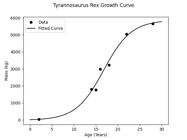
Fitted Tyrannosaurus Growth Curve

Again, just by visually inspecting this we can see that this is a very reasonable regression curve for the data!

Analysis

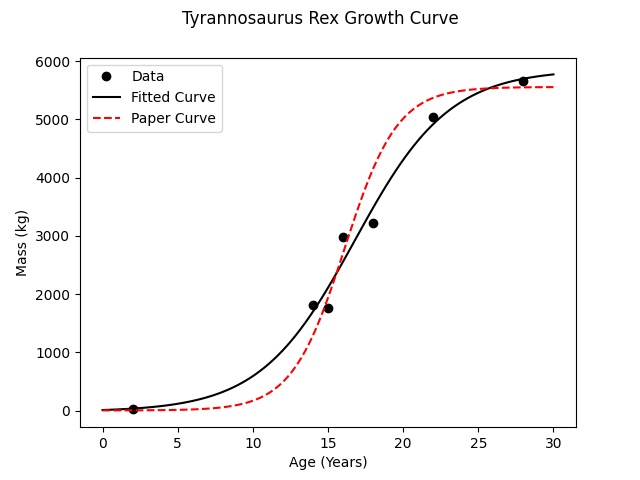
This is pretty fantastic - we were very quickly and easily able to fit a curve to the data! Unfortunately, as you may have noticed, the parameters that we found are not those found in the parper. In fact, we can plot the values that they gave against ours to see the difference:

Tyrannosaurus Growth Curve - Fitted Against Paper Parameters

 import numpy as np
 import pandas as pd
 import matplotlib.pyplot as plt

 from scipy.optimize import curve_fit

 def logistic(x, A, k, x_0, offset) -> float:
     expected = A / (1 + np.exp(-k * (x - x_0))) + offset
     return expected

 df = pd.read_csv('./tyrannosaurus_growth_table.csv', dtype={'age': np.double, 'mass': np.double})

 paper_values = [5551, 0.57, 16.1, 5]

 popt, pcov = curve_fit(logistic, df.age, df.mass, p0=paper_values)
 A, k, x_0, offset = popt

 # for plotting the fitted curve
 ages = np.linspace(0, 30, 101)
 masses = logistic(ages, *popt)
+paper_masses = logistic(ages, *paper_values)

 fig, ax = plt.subplots()
 fig.suptitle("Tyrannosaurus Rex Growth Curve")
 ax.plot('age', 'mass', 'ko', data=df, label="Data")
 ax.plot(ages, masses, 'k-', label="Fitted Curve")
+ax.plot(ages, paper_masses, 'r--', label="Paper Curve")
 ax.set_xlabel('Age (Years)')
 ax.set_ylabel('Mass (kg)')
 ax.legend()
-fig.savefig("tyrannosaurus_growth_curve.jpg")
+fig.savefig("tyrannosaurus_growth_curve_with_paper.jpg")

I may be biased, but the curve that we found seems to fit the data better. In fact, we can say empirically that it does - if you find the sum of mean squared errors for our fitted curve against the one from the paper, you find a higher sum of errors for the paper, which means that ours is a better fit to the data.

But why is this the case? The authors of the paper are clearly very intelligent and fitting a logistic curve to data is not exactly a difficult process, even accounting for the fact that 2004 was a great many years ago.

It turns out that I was not the only person who had some trouble replicating the results; (Myrhold, 2013) also noted that the published regression equations were not the best fit (for the Tyrannosaurus). In response, Erickson, et. al. published a corrigendum explaining their choices, which basically boil down to the fact that the fitted regression models produces values, especially for newly hatched or very old individuals, which are biologically infeasible. For instance, they noted that a regression equation produced masses at hatching (54kg) which is impossible, due to the nature of egg-laying.

And frankly, none of that is terribly important. A (the?) main question which Erickson, et. al. were trying to answer was how tyranosaurs attained thir massive sizes - either by growing faster or growing longer. In all of the analyses, the conclusion was the same - rather than growing for longer in order to attain their mazimum size, they grew more quickly.

Next Steps

There is obviously lots that we could do to further this analysis! One thing that stood out to me is that there is not a lot of time given to the uncertainty inherent in the measurements. In particular, there is a great deal of uncertainty in the estimates of the body masses, and none of that was reflected in the results. In addition, the selection of parameters to constrain the biological infeasability of the results made it harder to replicate the results. It would have been interesting to redo the analysis using a Bayesian framework, where the assumptions (e.g. 5kg at hatching) could have been encoded as strong priors on the parameters rather than fixing them in the analysis. In fact, that approach would also lend itself to an analysis incorporating the uncertainty in the masses!

Perhaps that will be something fun to do later…

Conclusion

SciPy’s curve_fit function allows you to fit an (almost) arbitrary regression function to observed data by generating optimal values for the function parameters. We used this first to perform a simple linear regression, and then to fit a logistic growth curve for Tyrannosaurus rex.

Mathsy Coding