Bayesian Ranking

Developing a way to assess the quality of players given the results of the games that they play

The purpose of this is to construct some sort of ranking given a series of pairwise comparisons, as well as an extension where the data is presented not as a series of one-on-one contests, but as a ranked order instead.

Theory and Simple Application

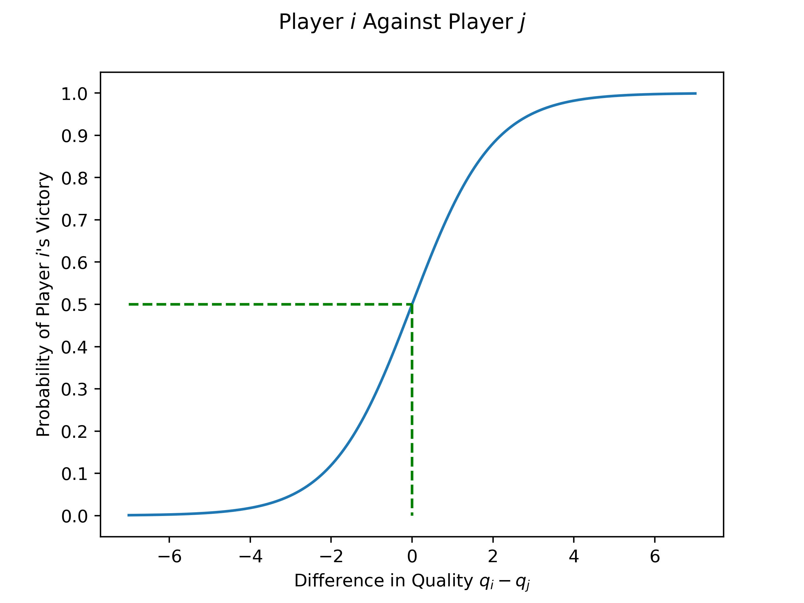
Let’s start with the basic idea. Imagine that you have some things that you want to rank. These could be movies, people, shapes - anything at all, as long as any two of them can be compared. For now, let’s make this concrete: imagine that we are ranking players playing tennis. We assume that each player has some sort of inherent quality $q_i$, and that if player $i$ plays against player $j$, the probability of player $i$ winning is given by the logistic curve

Let’s take a look at the graph:

import matplotlib.pyplot as plt
import numpy as np

fig, ax = plt.subplots()
diffs = np.linspace(-7, 7, 201)
probs = 1 / (1 + np.exp(-diffs))
ax.plot(diffs, probs) # the logistic curve

# This is to illustrate the when the qualities are the same (difference is 0), there is a probability of 0.5 of victory
ax.plot([-7, 0], [0.5, 0.5], 'g--')
ax.plot([0, 0], [0.5, 0], 'g--')

ax.set_yticks(np.linspace(0, 1, 11))
ax.set_xlabel("Difference in Quality $q_i - q_j$")
ax.set_ylabel("Probability of Player $i$'s Victory")
fig.suptitle("Player $i$ Against Player $j$")
fig.savefig('logistic_curve.png', dpi=400)

For the diagram, we can see that this way of calculating the probability of victory is at least reasonable. If player $i$ is much better than player $j$ (difference is large and positive), then the proability of their victory is close to 1, as you would expect. Similarly, if player $i$ is much worse that player $j$ (difference is large but negative), then the probability of their victory is close to zero. Finally, if the two players are equally matched (difference is 0), then the probability of victory is $50\%$.

The model that we are using is a variant of the Bradley-Terry model, which has many and varied uses.

Implementing the Model

Let’s implement the model using a Beysian framework! We’ll use PyMC to do the actual calculations, but the model itself looks like

Each game between players $i$ and $j$ is a Bernoulli trial, where the probability of victory is given by the logistic curve at the difference in the qualities. As a prior, we asssume that each player’s quality is given by a standard normal. If we were using actual data, we might modify the prior based on the player’s prior record or somesuch, but for now let’s start with this.

For this first implementation, let’s assume that we have three players with qualities 1, 0, and -1. Each player will play 100 games against each other player. We’ll generate the data, implement that model, then graph the results to see if we can recover the initial results.

import numpy as np
import pandas as pd
import matplotlib.pyplot as plt
import pymc as pm
from scipy.stats import bernoulli, gaussian_kde

# player name : quality
qualities = dict(A=1, B=0, C=-1)
players = list(qualities.keys())
num_games = 100

data = pd.DataFrame({"Player i":[], "Player j": [], "result": []})
for player_i in players:
    for player_j in players[players.index(player_i) + 1:]:
        prob_victory = 1 / (1 + np.exp(-(qualities[player_i] - qualities[player_j])))
        new_results = pd.DataFrame({"Player i": [player_i] * num_games, "Player j": [player_j] * num_games, "result": bernoulli.rvs(prob_victory, size=num_games)})
        data = pd.concat([data, new_results], ignore_index=True)

# convert the names of the players to their index - this is for the PyMC model we're about to use
data["Player i index"] = data.apply(lambda row: players.index(row["Player i"]), axis=1)
data["Player j index"] = data.apply(lambda row: players.index(row["Player j"]), axis=1)

# Now the model implementation
with pm.Model() as rank_model:
    quality = pm.Normal("quality", mu=0, sigma=1, shape=3)
    diffs = quality[data["Player i index"]] - quality[data["Player j index"]]
    prob_win = pm.math.sigmoid(diffs)
    results = pm.Bernoulli("results", prob_win, observed=data["result"])
    trace = pm.sample(tune=1000, return_inferencedata=False)

#Now let's plot these to see if we get the expected results:

quality_samples = trace.get_values("quality")
quality_samples.shape
samples = [[], [], []] # player 1, player 2, player 3
for index in [0, 1, 2]:
    for draw in quality_samples:
        samples[index].append(draw[index])
kdes = [gaussian_kde(collected_samples) for collected_samples in samples]

fig, ax = plt.subplots()
qs = np.linspace(-3, 3, 201)
for index, kde in enumerate(kdes):
    results = kde(qs)
    ax.plot(qs, results, label=f"{players[index]} - Quality {qualities[players[index]]}")
for player_quality in qualities.values():
    ax.axvline(player_quality, color="black", linestyle='--')
ax.set_xlabel("Quality")
ax.set_ylabel("Probability Density")
fig.suptitle("Ranking Results")
fig.legend(framealpha=1)
fig.savefig('initial_ranking.png', dpi=400)

Auto-assigning NUTS sampler...
Initializing NUTS using jitter+adapt_diag...
Multiprocess sampling (4 chains in 4 jobs)
NUTS: [quality]

Sampling 4 chains for 1_000 tune and 1_000 draw iterations (4_000 + 4_000 draws total) took 7 seconds.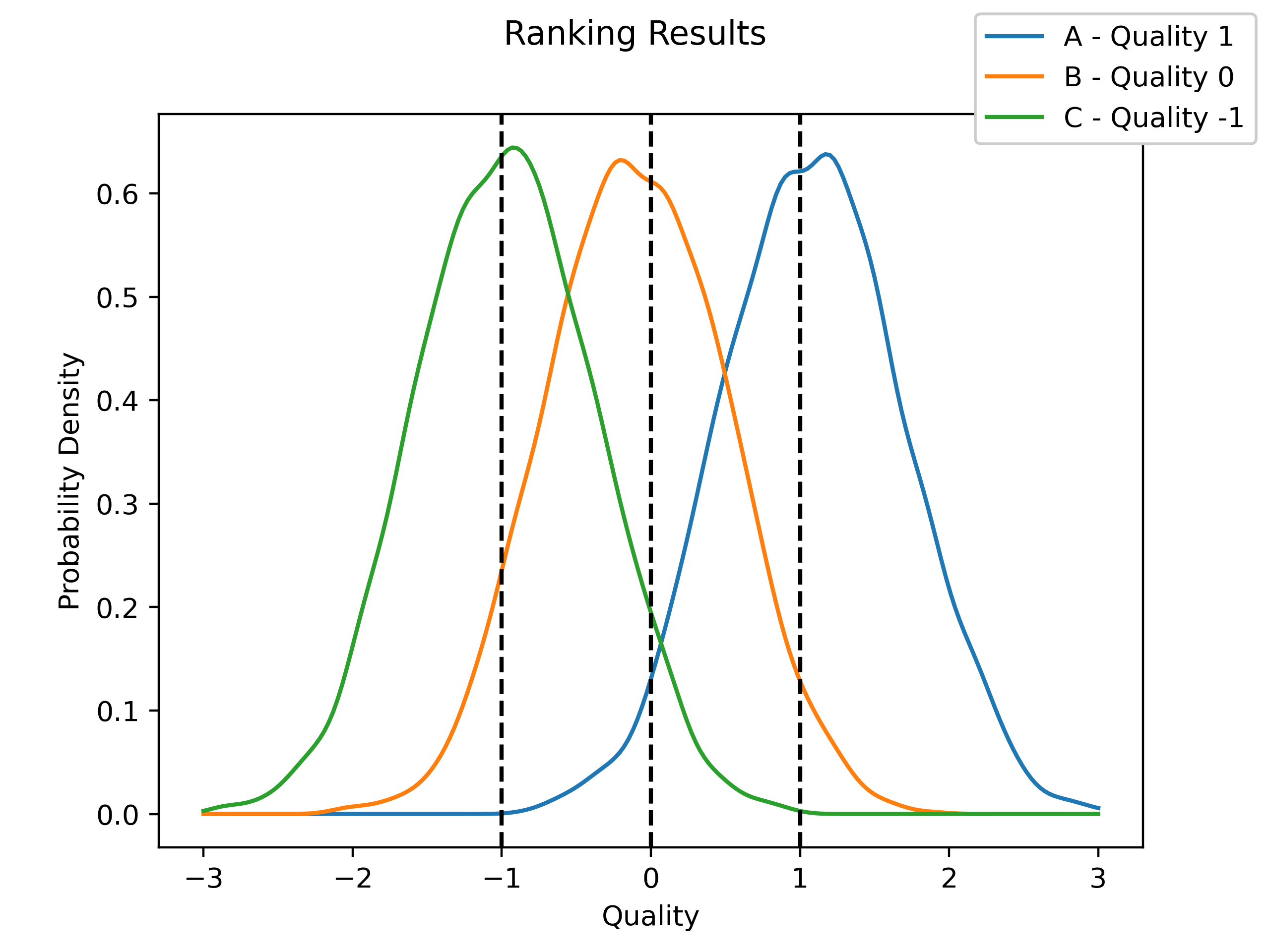

From this, we can see that our model is doing a good job of finding the original values. It looks like our method works!

A Further Application - Qualities from Rankings

Let’s try to extend this one step. Imagine that instead of one-on-one games, the data that we have is in fact a ranking of the players. Our raw data now looks like [A, B, C] to indicate that A is the best, followd by B, and then C. Of course, different “judges” may give slightly different rankings, but we would like to be able to establish an estimate for the underlying qualities regardless.

It turns out that this is in fact very simple! A ranking of [A, B, C] can be viewed as a set of three games: A against B (which A won), A against C (which A won), and B against C (which B won). In general, we can decompose a ranking of $n$ players into $n(n-1) / 2$ separate games. Let’s write a function which can automate this process:

from typing import List
import pandas as pd

def ranking_to_individual_games(ranking: List[str]) -> pd.DataFrame:
    """ Returns a DataFrame with columns 'Player i', 'Player j', and 'result' """
    data = pd.DataFrame({"Player i": [], "Player j": [], "result": []})
    for player_i in ranking:
        for player_j in ranking[ranking.index(player_i) + 1:]:
            new_row = pd.DataFrame({"Player i": [player_i], "Player j": [player_j], "result": [1]})
            data = pd.concat([data, new_row], ignore_index=True)
    return data

An Example

Again, let’s generate some data to see if our model is strong enough to recover the initial values. In order to do so, we will generate some rankings from players with a known (but not fixed) quality. Just as in the last case, we’ll generate the data, run the model, and the graph the results to see if we can recover the initial data.

import numpy as np
import matplotlib.pylab as plt
import pandas as pd
import pymc as pm
from scipy.stats import norm, gaussian_kde
from typing import List

def ranking_to_individual_games(ranking: List[str]) -> pd.DataFrame:
    """ Returns a DataFrame with columns 'Player i', 'Player j', and 'result' """
    data = pd.DataFrame({"Player i": [], "Player j": [], "result": []})
    for player_i in ranking:
        for player_j in ranking[ranking.index(player_i) + 1:]:
            new_row = pd.DataFrame({"Player i": [player_i], "Player j": [player_j], "result": [1]})
            data = pd.concat([data, new_row], ignore_index=True)
    return data

# these are now distributions because we're going to draw from them later to determine the rank order for a given "judgement"
qualities = dict(A=norm(1, 1), B=norm(0, 1), C=norm(-1, 1))
players = list(qualities.keys())
num_rankings = 1000

all_rankings = []
for _ in range(num_rankings):
    results = {player: qualities[player].rvs() for player in qualities}
    ranking = sorted(results, key=results.get, reverse=True)
    all_rankings.append(ranking)

# now generate the individual games
games_data = pd.DataFrame()
for ranking in all_rankings:
    games_data = pd.concat([games_data, ranking_to_individual_games(ranking)], ignore_index=True)

# convert the names of the players to their index (again)
games_data["Player i index"] = games_data.apply(lambda row: players.index(row["Player i"]), axis=1)
games_data["Player j index"] = games_data.apply(lambda row: players.index(row["Player j"]), axis=1)

with pm.Model() as ranking_model:
    quality = pm.Normal("quality", mu=0, sigma=1, shape=3)
    diffs = quality[games_data["Player i index"]] - quality[games_data["Player j index"]]
    prob_win = pm.math.sigmoid(diffs)
    results = pm.Bernoulli("results", prob_win, observed=games_data["result"])
    trace = pm.sample(tune=1000, return_inferencedata=False)

quality_samples = trace.get_values("quality")
samples = [[], [], []]
for index in [0, 1, 2]:
    for draw in quality_samples:
        samples[index].append(draw[index])
kdes = [gaussian_kde(collected_samples) for collected_samples in samples]

# again, graph the results
fig, ax = plt.subplots()
qs = np.linspace(-3, 3, 201)
for index, kde in enumerate(kdes):
    results = kde(qs)
    ax.plot(qs, results, label=players[index])
ax.set_xlabel("Quality")
ax.set_ylabel("Probability Density")
fig.suptitle("Ranking Results")
fig.legend(framealpha=1)
fig.savefig('ranking_from_ranked_data.png', dpi=400)

Auto-assigning NUTS sampler...
Initializing NUTS using jitter+adapt_diag...
Multiprocess sampling (4 chains in 4 jobs)
NUTS: [quality]

Sampling 4 chains for 1_000 tune and 1_000 draw iterations (4_000 + 4_000 draws total) took 7 seconds.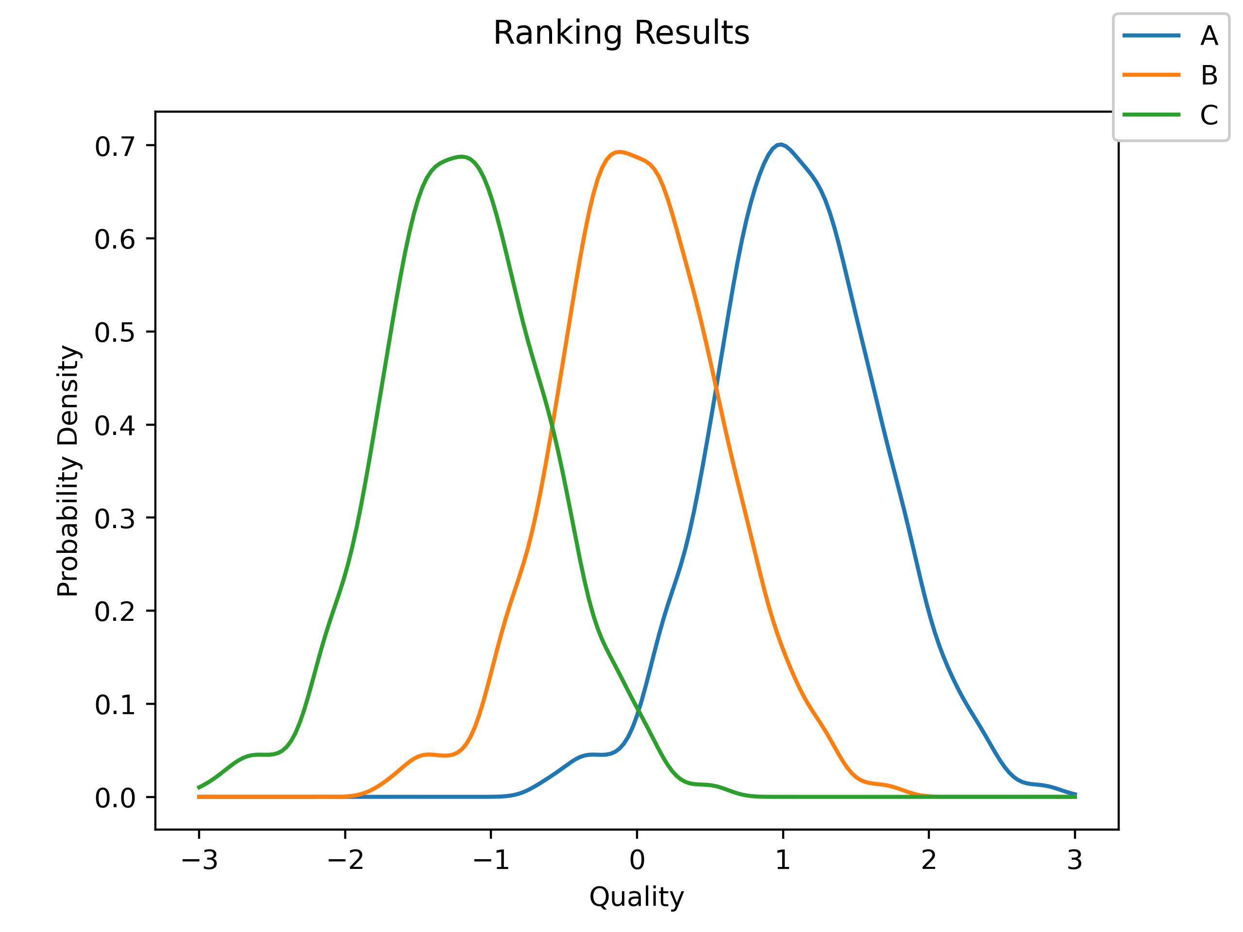

Once again, our model was able to recover the initial values with a high degree of fidelity, although the results are somewhat more dispersed around the true values then when we had the individual games.

Conclusion

So there we have it! In this post we examined how to develop a ranking of players, given either a set of individual contests or a set of rankings which we then decomposed into equivalent ‘individual games’.

Bibliography and Sources

• Learning to Rank the Bayesian Way - Dr. Robert Kubler
• Bradley-Terry Model - Wikipedia
• Bernoulli distribution