Inferring Extinction from Sighting Data

Working through the details of Sorlow's 1993 paper "Inferring Extinction from Sighting Data"

As part of my attempt to understand more about the papers I’m reading, I’ve decided to work through all of the calculations of some of them to see if I can reproduce them. Today, I’m going to take a look at a 1993 paper by Andrew Solow entitled “Inferring Extinction from Sighting Data”. This paper is about how confident we can be in our belief that an animal has gone extinct, based on a previous record of sightings.

One of my goals with this is to lay out the steps in enough detail that anyone interested can follow along. Necessarily, that will mean that I will try not to skip steps that people with more experience would consider obvious.

The Problem and Situation

The basic problem that the paper is trying to solve is as follows. Imagine that you have an animal of some sort, which you know about only from occasional sightings. Maybe this animal is rare, maybe its habits keep it from people (e.g. it is nocturnal), or maybe it just lives somewhere very remote. Regardless, at some point you stop seeing it. If that is the case, then at what point can you decide that in fact the animal is extinct? How confident can you be in the fact that it is extinct?

To make things easier (=tractable), let’s assume that the sightings are the realization of a Poisson process. We will consider the observations as having occurred over the time interval $(0, T)$ (where we can assume that $0$ is the beginning of observations and $T$ is the present - for simplicity). Then the observation data looks like $\vec{t}=(t_1, t_2, \ldots, t_n)$. For instance, if I make observations of ants in my house for a year (12 months), then my total time interval might look like $(0, 11)$ and my observation data might look like $\vec{t}=(1, 4, 5, 8)$ to show that I saw ants in my house in February, May, June, and September.

However, we are interested in extinction time. Let’s say that the population of interest goes extinct at time $T_E$. It may be that $T_E \in (0, T)$, in which case the population is already extinct. However, it could also be the case that $T_E \ge T$, in which case the population either just went extinct or will do so in the future. As far as we are concerned, these cases are the same.

In that case, the rate function for the Poisson process generating the sightings is

We don’t know the value of either $m$ or $T_E$, but we are very interested in $T_E$!

Solow presents two methods: one based on frequentist statistics and hypothesis testing, and the other based on Bayesian statistics.

He also uses a concrete example: the extinction (or not?) of the Carribean monk seal (using information found in LeBoeuf et al (1986). Let’s follow along, using that same data.

import numpy as np

current_date = 1992 # although the paper was published in 1993, it must have been written in 1992 since that is what Solow uses
sighting_dates = np.array((1915, 1922, 1932, 1948, 1952)) # from LeBoeuf (1986)
normalizing_constant = sighting_dates.min()
normalized_dates = sighting_dates - normalizing_constant # we want to start everything at 0
T = current_date - normalizing_constant
normalized_dates, T

(array([ 0,  7, 17, 33, 37]), 77)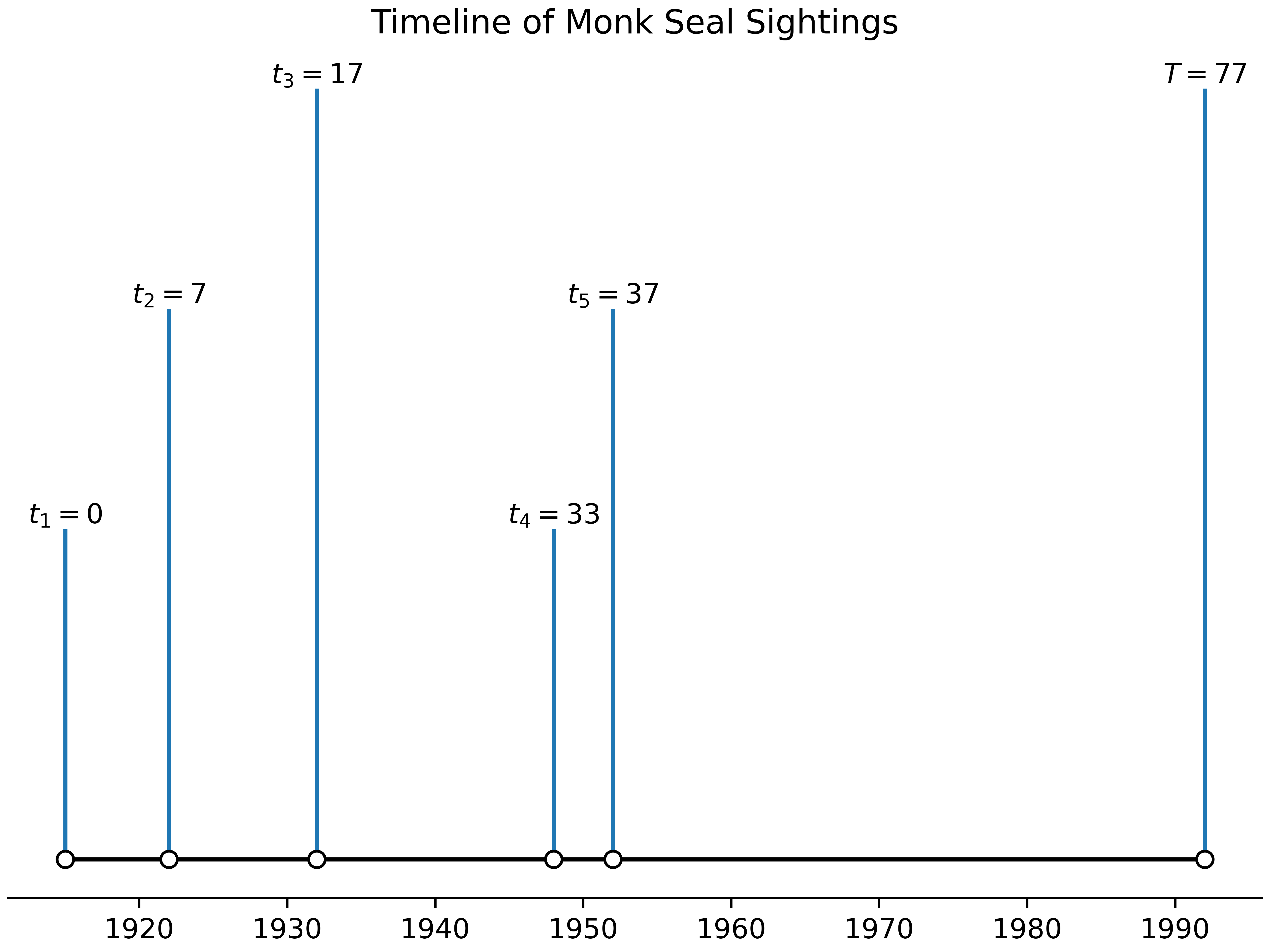

import numpy as np
import matplotlib.pyplot as plt

# data
current_date = 1992 # although the paper was published in 1993, it must have been written in 1992 since that is what Solow uses
sighting_dates = np.array((1915, 1922, 1932, 1948, 1952)) # from LeBoeuf (1986)
normalizing_constant = sighting_dates.min()
normalized_dates = sighting_dates - normalizing_constant # we want to start everything at 0
T = current_date - normalizing_constant

# Visualizing (based on https://matplotlib.org/stable/gallery/lines_bars_and_markers/timeline.html)
dates = np.array([*sighting_dates, current_date])
labels = [f"$t_{index + 1}={normalized_date}$" for index, normalized_date in enumerate(normalized_dates)]
labels.append(f"$T={T}$")
fig, ax = plt.subplots(constrained_layout=True)

ax.set(title="Timeline of Monk Seal Sightings")

# draw the stems and label them - do this first so the lines are under the marker
levels = np.repeat(0.5, dates.shape) + np.array([0.2 * (i % 3 - 1) for i in range(len(labels))])
for date, label, level in zip(dates, labels, levels):
    ax.vlines(date, ymin=0, ymax=level)
    ax.annotate(text=label, xy=(date, level), verticalalignment="bottom", horizontalalignment="center")
ax.plot(dates, # x coords
        np.zeros(dates.shape), # fake y coords - all zeros
        '-o', # solid line, solid circular marker
        color='k', # black
        markerfacecolor='w', # make the markers look hollow
    )

ax.yaxis.set_visible(False)
ax.spines[['left', 'right', 'top']].set_visible(False)

plt.savefig('timeline.png', dpi=800)

As we can see, no one has seen a Monk seal in quite some time (remember: $T$ is the current date, and not a sighting) - just intuitively, it seems like it might be extinct! Let’s see how Solow approaches this more methodically.

The Frequentist Approach

Here we are going to test the null hypothesis $H_0: T_E = T$ (extinction has not occurred) against the alternative hypothesis $H_1: T_E < T$. (Remember that $T$ is the present).

Recall that a statistical hypothesis test of this form is done in the following way. We go forward as though the null hypothesis is true. Then we calculate the probability of seeing the data that we have under the null hypothesis. If this probability is incredibly unlikely (for whatever value of incredibly we choose to use), then we reject the null hypothesis in favour of the alternative hypothesis. If, however, the data is not terrible unlikely (again, by whatever standards we choose to use), then we grudgingly accept the null hypothesis (Walpole and Myers, 1985).

Let’s let $T_i$ be a random variable, of which the individual sighting $t_i$ is a realization. Conditional on the number of observations, $T_i$ is uniformly distributed over the interval $(0, T)$. That is, $T_i \sim \text{Uniform}(0, T)$; the probability density function of $T_i$ is $f(t) = \frac{1}{T}$ (Ghahramani 2005).

What does this mean? Simply that if the number of sightings is fixed (say at 5), and they are the realization of a Poisson process, then we expect the sightings to be uniformly distributed over the range. If that’s the case, then a natural statistic to use is the time of the most recent sighting, $T_n$. Recall that our test statistic is the one that we are going to use to decide whether the results that we see are “improbable enough”. In this case, having $T_n$ be too low (i.e. we haven’t seen the animal in too long) will allow us to reject the null hypothesis and decide that it has in fact gone extinct.

The probability that the most recent sighting is less than our actual most recent sighting, $t_n$, is

We want the probability of a type 1 error (that is, rejecting the null hypothesis when it is true) to be less than some predefined quantity $\alpha$. This $\alpha$ is also known as the level of significance (Walpole & Myers 1985). If we set $\alpha$ to some predefined value (commonly 0.05 or 0.01), then we can find the critical region for our last sighting, $t_n$. Recall that the critical region is the set of values (in this case, for $t_n$) where we will reject the null hypothesis (decide that extinction has occurred). The critical value is the one (or ones) that form the boundary of the critical region (Walpole & Myers 1985). The calculation for the critical value is as follows:

We can also think of this as the ratio of the last sighting to the total time $\frac{t_n}{T} = \alpha^{\frac{1}{n}}$. For instance, if we want a significance level of $5\% \to \alpha = 0.05$ and we have $n=10$ sightings, then we want $\frac{t_n}{T} = 0.05^{\frac{1}{10}} = 0.7411\dots$. In our case, that means that if our last sighting occurs earlier than 74% of the way through our study period, we reject the null hypothesis, and if it occurs later than 74% of the way through, then we accept it. This make sense intuitively - if we haven’t seen the population in a long time we are more likely to believe that it went extinct, whereas if we have seen it recently we are less likely to believe that it went extinct.

Let’s see what happens with our Monk seal data. First, we need to make a slight adjustment - we’re going to ignore the first point. Why is this? Well, the problem is that we don’t really have a good place to begin our observations. Thus, we’ll just pretend that we started observing at the first data point and just ignore it. That means that we are really working one fewer data point than we initially thought. Let’s see what we get:

alpha = 0.05
n = normalized_dates.shape[0] - 1 # removing the first one from consideration
t_n = normalized_dates[-1]
p_value = (t_n / T) ** n
print(f"p value = {p_value}")

p value = 0.05331433488215145

Which is generally considered pretty good evidence against the null hypothesis, and so we might consider that the Monk seal is extinct.

It turns out that use this same idea to define the power of our test. The power of a test is the probability that we will correctly reject the null hypothesis when our alternative hypothesis is true. In this case, our alternative hypothesis is that $T_E < T$. If that is true, then our values will be uniformly distributed on $(0, T_E)$ (instead of over $(0, T)$ as in the case where the null is true). If $T_E$ is less than our critical value $\alpha^{\frac{1}{n}}T$, then we will surely reject the null, since the last sighting must logically be inside our critical region. However, we may erroneously accept the null even if the extinction time $T_E$ is outside of the critical region.

As a concrete example, imagine a case with $\alpha=0.05$ and $n=10$. In that case, our critical region was the initial 74% of the study period - as long as the most recent observations occur outside of this region, we accept the null hypothesis of no extinction. However, say that the null hypothesis is incorrect, and the population actually went extinct 80% of the way through the study time. Now, if we see an observation in the region (74%, 80%) we will incorrectly accept the null hypothesis and believe that no extinction has taken place. However, it is certainly possible that even though the population exists in that (74%, 80%) interval, we never see it, and thus correctly reject the null hypothesis. So then to find the power of the test (the probability of correctly rejecting the null hypothesis), we need the probability that we will get the last observation time $T_n$ in the critical region (0, 74%). If the population went extinct at time $T_E = 0.8T$, then the observations are again uniformly distributed, but now with probability density $f(t) = \frac{1}{T_E} = \frac{1}{0.8T}$. Again, we can use the test statistic $T_N$, our lastest observation. Then the probability that we see $T_N$ in the critical region is

So if the population went extinct 80% of the way through the study period, then we still have a slightly greater than 45% chance of correctly rejecting the null hypothesis (determining that it went extinct).

More formally, we have

Thus, we can calculate our power as follows:

The Bayesian Approach

Recall that Bayes’ Theorem is that

In our context, we have data $\vec{t}$ and we are trying to find the probability that our null hypothesis ($H_0: T_E \ge T$) is true. We then get that

where

• $P(H_0 | \vec{t})$ is our posterior probability that our null hypothesis is true
• $l(\vec{t} | H_0)$ is the likelihood of our data, given that our null hypothesis is true
• $\pi$ is the prior probability of our null hypothesis - that is, the probability that the null hypothesis is true before we see the data
• $l(\vec{t})$ is the likelihood of seeing our data

For this situation, there are only two cases: either $H_0$ or $H_1$ are true. If the probability of $H_0$ is $\pi$, then the probability of $H_1$ must be $1-\pi$. Thus, we can also write that

and so by combining equations (1) and (2),

One criticism of the Bayesian approach is that the prior likelihood $\pi$ will tend to influence the results, more strongly with less data and less strongly with more. One way to sidestep this is to use the Bayes factor. For two hypotheses $H_0$ and $H_1$, the Bayes factor is the ratio of the probabilities of seeing the data under $H_0$ against $H_1$. You can think of it as a measure of how strongly the data supports one hypothesis over the other. In our case, the Bayes factor $B(\vec{t})$ is

If the Bayes factor is greater than 1 then the data support $H_0$ more strongly than $H_1$; if it is less than 1 then the reverse is true.

For any particular prior likelihood $\pi$, we can recover the probability $P(H_0|\vec{t}) = \frac{1}{1 + \frac{1-\pi}{\pi B(\vec{t})}}$

First

And so we have

In order to calculate the Bayes factor, we need $l(\vec{t}|H_0)$ and $l(\vec{t}|H_1)$.

Starting with the likelihood under the prior, $l(\vec{t}|H_0) = \int_0^\infty l(\vec{t}|m)dP(m)$, where here we are integrating over our prior probability of the rate $m$ ($P(m)$ is the prior probability of $m$).

Under $H_0$, the data that we see are the realization of a Poisson process. Again, under the condition that the number of observations is fixed, then these are distributed as per a uniform distriubtion with probability density $f(t) = \frac{1}{T}$. This means that the likelihood of our data $l(\vec{t}|H_0) = \frac{n!}{T^n}$.

This idea actually took me a while to wrap my head around - naively, I would have thought that it was just $\frac{1}{T^n}$ (since that is $P(T_1=t_1) \ast P(T_2=t_2) \ast \dots \ast P(T_n=t_n)$). However, that misses the fact that although we are ordering the data, the uniform distribution does not. For the uniform distribution, getting values of 1987, 1988, and 1989 is exactly the same probability of getting 1988, 1989, and 1987 - we are the ones that are ordering them. Thus, since there are $n!$ ways of generating our data (in whatever order), and each has probability $\frac{1}{T^n}$, the final likelihood of $\frac{n!}{T^n}$.

As a more concrete example: imagine we roll a dice three times and then order the results. We get 1, 2, and 3. The probability that we got that is not $\frac{1}{6^3}$ - that would be the probability that we get first the 1, then the 2, then the 3. However, since we are ordering the results ourselves, if we had gotten a 3, then a 1, then a 2, we still would have seen the same results. We know that are getting a 1, 2, and 3 in some order. Each way of generating a 1, a 2, and 3 has probability of occurring of $\frac{1}{6^3}$, and there are 6 ($=3!$) ways of arranging these, the final probability is $\frac{3!}{6^3}$.

So to get back to our likelihood $l(\vec{t}|H_0)$:

In order to calculate the Bayes factor, we need $\int_0^\infty l(\vec{t}|H_0) dP(m)$. Solow uses the uninformative prior given by $dP(m) = \frac{1}{m}dm$. Subbing this in, we get

Wait, what? How did we solve that integral? Well, the honest answer is that I plugged it into Wolfram Alpha. However, it turns out that it’s actually not that hard. The trick is to realize that the gamma function looks a lot like our integral, and has a defined solution: $\int_0^\infty m^{n-1}e^{-m}dm = \Gamma(n)$. Thus, by making the variable substitution $t = mT$, we have

And so we have calculated $l(\vec{t}|H_0)$.

Now we need $l(\vec{t}|H_1)$. This one will be a little more complicated, since under $H_1$ we actually have two parameters we need to integrate over: the rate $m$ and the time of extinction $T_e$. However, the basic idea is the same as above:

Phew! So finally, we have both propabilities that we need, and can calculate the Bayes factor:

If we use the data that we have, we can plug that in and say that

bayes_factor = (n - 1) / ((T / t_n) ** (n - 1) - 1)
print(f"Bayes Factor: {bayes_factor}")

Bayes Factor: 0.3743939095299103

Which means that our evidence support $H_1$ (extinction) about three time as much as it does $H_0$ (no extinction). This is generally considered to be fairly weak evidence for $H_1$, and so we are slightly convinced that the Monk seal is extinct.

We can also calculate the probability that $H_0$ is true and the seal is not extinct. Going back to our earlier formula and starting with a likelihood $\pi=0.5$,

pi = 0.5
p_h0 = 1 / (1 + ((1 - pi) / (pi * bayes_factor)))
print(f"Probability of H_0 (No Extinction): {p_h0*100:.2f}%")
print(f"Probability of H_1 (Extintion): {(1-p_h0)*100:.2f}%")

Probability of H_0 (No Extinction): 27.24%
Probability of H_1 (Extintion): 72.76%

So under this model, there is about a 72.8% chance that the seal is extinct.

Discussion

First of all: this was a lot of fun! It has been a long time since I did any real probability / statistics work like this, and it was really interesting to go and pull out some of that knowledge. Although it took me a long, long time to work through, especially considering that the paper itself is only about four pages long, it reminded me of both how frustrating mathematics can be and how great it feels when you finally figure out the solution.

Although my formal training in statistics (such as it is) is only from a frequentist perspective, I found myself not really enjoying that aspect of the paper. The mental model of null hypothesis and then rejecting or failing to reject it is feeling a bit foreign to me. I much preferred the Bayesian approach, although to be honest most of my experice with that has come from a computational perspective (that is, getting the computer to do the calculations). To be honest, it’s something that I want to get better at. Although I can recognize those integrals for the likelihood as being correct, I probably wouldn’t be able to come up with them on my own. Similarly, I am not sure how the priors (as stated in the paper) relate to the way that I would generally formulate them (in terms of the raw prior rather then $dP$). But I’m excited to learn!

From a brief glance at the literature, it looks like there are lots of papers, both by Solow and others, that explore the idea of inferring extinction in more detail. It should be fun to look through those and see how they differ from this model!

Bibliography / Sources

• Ghahramani, S. (2005). Fundamentals of Probability: With Stochastic Processes, Third Edition (3rd edition). Chapman and Hall/CRC.
• LeBoeuf, B. J., Kenyon, K. W., & Villa-Ramirez, B. (1986). The Caribbean Monk Seal Is Extinct. Marine Mammal Science, 2(1), 70–72. https://doi.org/10.1111/j.1748-7692.1986.tb00028.x
• Solow, A. R. (1993). Inferring Extinction from Sighting Data. Ecology, 74(3), 962–964. https://doi.org/10.2307/1940821
• Walpole, R. E., & Myers, R. H. (1985). Probability and Statistics for Engineers and Scientists. Macmillan USA.