Logistic Growth with Harvesting

Analyzing the effects of different harvesting methods on a system described by logistic growth

(Most of this is based on Chapter 1 of (Murray 2002).

In an earlier post, I examined the behaviour of a population whose growth was given by the following equation.

Where $r$ is the growth rate and $K$ is the carrying capacity. In this post, we’ll examine what happens when we add harvesting to this equation. We’ll begin with constant effort harvesting, and then move on to constant yield harvesting. We’ll take a look at their long-term behaviours, their sensitivies to small perturbations, and make some final comments about possible implications for management of stocks.

Constant Effort Harvesting

Imagine that we want to harvest a population which otherwise would obey the logistic growth model. One way that we could model the additional harvesting is with some effort parameter $E$. This parameter could somehow represent how much time we are putting into it, how many boats we’re sending out, or something along those lines. Then the new equation which the population obeys would be

As indicated, the product of the population $N$ and the effort $E$ would be the yield.

The first question that we should probably ask is: what are the equilibrium populations here? Clearly $N=0$ is one, and the other is given by

Since this is the only equilibrium that we care about, let’s give it a special name:

Clearly, this only makes sense if $E < r$. Considering that $r$ is the unrestricted growth rate, if we are harvesting the population faster than it can grow under even ideal circumstances, then it clearly has no hope.

At this equilibrium population, the yield that we get is

So then the question becomes: what sort of effort should we put in to get the maximum yield?

At this effort, the maximum sustainable yield $Y_M$ is

Dynamics

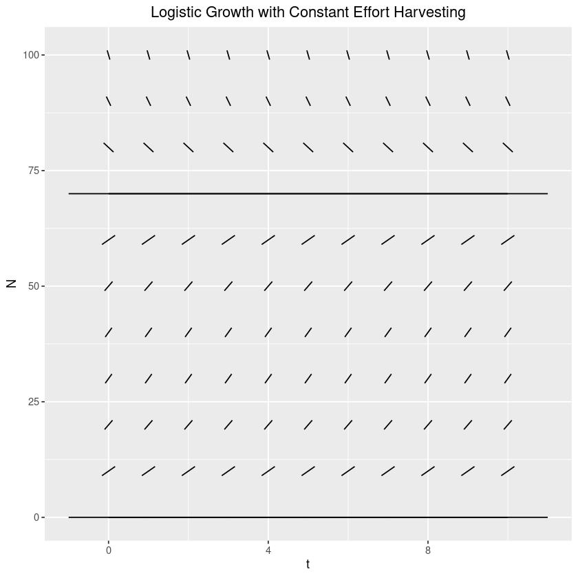
We’d like to get a feel for the dynamics of the behaviour around the equilibrium point. The first thing that we should do is to create a slope field. For us, let’s start with $r=1$, $K=100$, and $E=0.3$. Note that $E < \frac{r}{2}$, our highest yielding effort.

library(ggplot2)
library(latex2exp)

generate_slope_field <- function(xs, ys, diff, length=1) {
    df <- expand.grid(x=xs, y=ys)
    df$m <- diff(df$x, df$y)
    df$theta <- atan(df$m)
    df$xstart <- df$x - 0.5 * length * cos(df$theta)
    df$ystart <- df$y - 0.5 * length * sin(df$theta)
    df$xend <- df$x + 0.5 * length * cos(df$theta)
    df$yend <- df$y + 0.5 * length * sin(df$theta)

    graph <- ggplot(df) + geom_segment(aes(x=xstart, y=ystart, xend=xend, yend=yend))
    return(graph)
}

diff <- function(t, N) {
    r = 1
    K = 100
    E = 0.3
    return(r * N * (1 - N / K) - E * N)
}
ts <- seq(0, 10, by=1)
Ns <- seq(0, 100, by=10)
graph <- generate_slope_field(ts, Ns, diff, length=2)
graph +
    xlab(TeX("$t$")) +
    ylab(TeX("$N$")) +
    ggtitle("Logistic Growth with Constant Effort Harvesting") +
    theme(plot.title=element_text(hjust=0.5))

Note that from this we see that the behaviour looks basically identical to that of the regular unharvested logistic - the equilibrium at $N=0$ is unstable, while that at $N_h(E)$ is stable. Just to be safe though, let’s take a look at this algebraically (around $N_h$).

Set $\delta = N - N_h$, the difference between the current population and the equilibrium one. Then $\frac{d\delta}{dt} = \frac{dN}{dt} - \frac{dN_h}{dt} = \frac{dN}{dt} = f(N)$. Linearizing about $N_h$ gives us

Since in the region around the equilibrium point $\delta$ behaves approximately as an exponential, we can see that this equilibirum point is stable if $E < r$ and unstable otherwise.

Now let’s consider the time to recovery after the population is perturbed by some small amount from its equilibrium state. Since these systems behave basically like the exponential in a small region around the equilibirium point, a natural way to characterize the time to recovery is in terms of the coefficient of the exponent of the exponential. That is, if $N \approx e^{at}$, then the coefficient of interest is $a$, and the ‘time to recovery’ is $\frac{1}{a}$ - the time it takes for the population to change by a factor of $e$.

To start with, let’s consider the case where $E = 0$ - the standard logistic curve. In that case, the deviation from the equilibrium at $N = K$ is given by $\frac{d}{dt}(N - K) \approx -r (N - K) \to N - K \approx e ^ {-rt}$ (eq. 2), and so the recovery time is $O\left( \frac{1}{r} \right)$. When $E \in (0, r)$, then by the exact same process we have the recovery time is $O\left( \frac{1}{E - r} \right)$.

Consider the time to recovery $T_r(E)$ as a function of the effort $E$ that we put into harvesting. Rather than consider the absolute time to recovery, we can instead consider the ratio of the recovery time when we are harvesting to what it would be if we weren’t: that is, we can take a look at $T_r(E) / T_r(0)$.

From this, we can clearly see that in the limit as $E \to 0$, $T_r(E) \to \frac{1}{r}$ (as expected), and when $E \to r$, $T_r(E) \to \infty$, which again makes sense.

When we are harvesting at our maximum sustainable yield, that means the $E = \frac{r}{2}$ and so $T_r(E) / T_r(0) = O\left( \frac{1}{1 - \frac{\frac{r}{2}}{r}}\right) = O\left( \frac{1}{1 - \frac{1}{2}} \right) = O(2)$, so it takes the population roughly twice as long to recover as it would with no harvesting pressure at all.

But now let’s look at this a different way. If we are actually harvesting a population, we don’t know $E$, the proxy for effort. Instead, we see $Y$, the yield! So now let’s re-write our ratio of recovery times in terms of the observed yield $Y$ instead of the unobserved effort $E$.

Solving the quadratic for $E$, we have

And then by substituting into our ratio of recovery times,

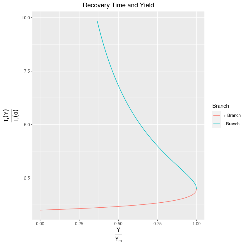
Perhaps seeing this visually will help in our analysis:

y_ratio <- seq(0, 1, by=0.005)
get_positive_branch <- function(y_ratios) {
    return(2 / (1 + sqrt(1 - y_ratios)))
}
get_negative_branch <- function(y_ratios) {
    return(2 / (1 - sqrt(1 - y_ratios)))
}
df <- data.frame(y_ratio=y_ratio)
df['+ Branch'] <- get_positive_branch(df$y_ratio)
df['- Branch'] <- get_negative_branch(df$y_ratio)
melted <- cbind(df['y_ratio'], stack(df[c('+ Branch', '- Branch')]))
melted = melted[melted$values < 10,]

ggplot(melted, aes(x=y_ratio, y=values, colour=ind), ) +
    geom_line() +
    ylab(TeX("$\\frac{T_r(Y)}{T_r(0)}$")) +
    xlab(TeX("$\\frac{Y}{Y_m}$")) +
    ggtitle("Recovery Time and Yield") +
    theme(plot.title=element_text(hjust=0.5)) +
    guides(colour=guide_legend(title="Branch"))

One thing that becomes immediately clear from this diagram is that for a given yield (or rather, ratio $Y/Y_m$, which amounts to the same thing), we can get that yield using a relatively small amount of effort and with a relatively quick recovery time (the positive branch), or we can be there with a large amount of effort and a long recovery time (the negative branch). Clearly, we would rather be on the positive one! Here’s where things get tricky though. Imagine that you have somehow ended up on the negative branch and want to get a higher yield. Then, paradoxically, you need to decrease the amount of effort that you are putting into harvesting!

Constant Yield Harvesting

Now let’s consider another model of harvesting - one where you aim for a constant harvest, rather than a constant effort. In practical terms, this might look like setting the entire allowable catch for an entire fishing fleet to 100 tonnes (constant harvest) rather than legislating that the season is open for only one month (constant effort). How does our analysis change in that case?

Well first, let’s write down the equation governing this scenario. If our constant harvest (yield) is $Y_0$, then we have

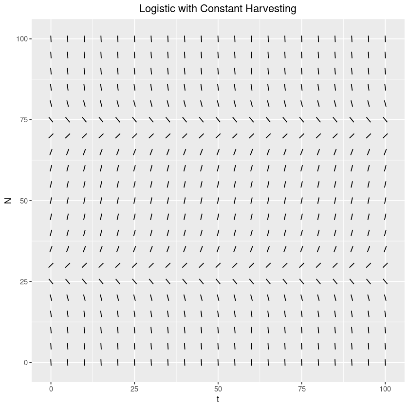
Again, let’s get a general feel for how this system behaves by looking at the slope field:

diff <- function(t, N) {
    K <- 100
    r <- 1
    Y_0 <- 20
    return(r*N*(1 - N / K) - Y_0)
}
t <- seq(0, 100, by=5)
N <- seq(0, 100, by=5)
graph <- generate_slope_field(t, N, diff, length=2)
graph +
    ylab("N") +
    xlab("t") +
    ggtitle("Logistic with Constant Harvesting") +
    theme(plot.title=element_text(hjust=0.5))

From examining the slope field diagram, it looks like there are two equilibrium points. The lower one seems unstable, while the upper appears stable. Let’s call the lower equilibrium $N_1$ and the upper one $N_2$. If the population ever reaches a level below $N_1$, then it will decrease. In fact, in contrast to the base logistic system, which experiences exponential decay, this system will reach $N=0$ in a finite amount of time! To see why, notice that as $N \to 0$, $\frac{dN}{dt} \to -Y_0$. Thus, when we are close enough to $N=0$, we can say that

if at some $t_0$ we have that $N(t_0)=N_0$ is very small (so that our approximation holds), then $N \approx -Y_0 (t - t_0) + N_0$, which means that at time $t = t_0 + \frac{N_0}{Y_0}$, $N = 0$. So this actually decreases very quickly from this unstable equilibrium!

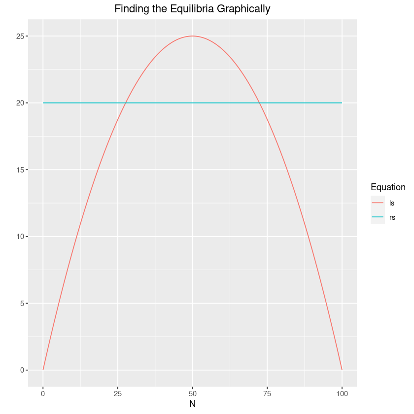
If we examine the equilibria in a slightly different light, we can see that this fact will have some pretty serious ramifications for the model. To see why, let’s examine the solution to the equilibrium points graphically. To do so, we’ll use the following:

K <- 100
r <- 1
Y_0 <- 20

N <- seq(0, 100, by=0.1)
df <- data.frame(N=N, ls=r*N*(1-N/K), rs=Y_0)
melted <- cbind(df['N'], stack(df[c('ls', 'rs')]))
ggplot(melted, aes(x=N, y=values, colour=ind)) +
    geom_line() +
    ylab("") +
    xlab("N") +
    ggtitle("Finding the Equilibria Graphically") +
    theme(plot.title=element_text(hjust=0.5)) +
    guides(colour=guide_legend(title="Equation"))

Since the left side is just the standard logistic, we know that its vertex appears at $\left(\frac{K}{2}, \frac{rK}{4} \right)$. Now consider what happens as we increase the yield. The two equilibrium points $N_1$ and $N_2$ will get closer and closer together. Now generally we will want to be at the higher, stable equilibrium $N_2$. However, as the equilibria get closer and closer together, it will become easier and easier to accidentally slip from one equilibrium to another, with disastrous consequences!

Now let’s take a look at the ratio of recovery times, $\frac{T_r(Y_0)}{T_r(0)}$. This really only makes sense for the stable equilibrium $N_2$, so our first step should probably be to find that analytically.

Just like before, we’ll set $\delta = N - N_2(Y_0)$. Then

Therefore, $\delta \propto e^{-r\sqrt{1 - \frac{4Y_0}{rK}}t}$, giving a time of recovery of $O\left( \frac{1}{r\sqrt{1 - \frac{4Y_0}{rK}}} \right)$. Since the time of recovery when $Y = 0$ is still $O\left( \frac{1}{r} \right)$, that gives us a ratio of

Now we have a problem - as $Y_0 \to Y_M$, the ratio of recovery time goes to infinity! Obviously this is not a great thing to have happen, and presents a contrast to the earlier constant effort model.

In fact, from this very simple analysis it seems clear that, both in terms of stability and recovery time, the constant effort model is superior. However, before I say anything else too strongly I should note that I have no practical experience in any sort of resource management, and there is an excellent chance that real populations would behave differently than either of the two models presented here, so any sort of conclusion we draw from this should be applied only with the greatest caution.

Conclusion

Although relatively simple, comparing and contrasting these two models allowed us to explore a variety of methods. We took a look at various approximation around equilibrium points, examined the stability through this lens, and further used it to make some conclusions about population recovery times from small perturbations. We were also able to make some conclusions about different harvesting strategies, although we should take these with a large grain of salt.

Sources

• Murray, J. D. (Ed.). (2002). Mathematical Biology: I. An Introduction (Vol. 17). Springer. https://doi.org/10.1007/b98868