A Simple Bayesian Workflow with PyMC

Jun 20, 2023

Going through a simple linear regression using PyMC3

In this post, I’m going to go through a simple process of performing a Bayesian linear regression, including an example workflow.

The Data

Because the purpose here is just to go through the process and fit the model, rather than any of the other interpretive work that goes into creating a model, we’ll start with known data.

import pymc3 as pm
import matplotlib.pyplot as plt
import arviz as az

m = 2
b = 1
x = np.linspace(-2, 2, 100)
true_y = m * x + b
observed_y = true_y + np.random.normal(loc=0, scale=1, size=len(x))

fig, ax = plt.subplots()
ax.scatter(x, observed_y, label="Observed")
ax.plot(x, true_y, label="True Values")
ax.set_xlabel('$x$')
ax.set_ylabel('$y$')
ax.legend()
ax.set_title('Observed and True Values')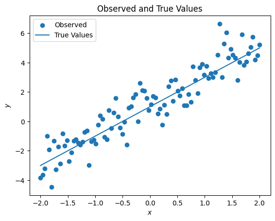

A plot of the true and observed values for a linear function.

The Model

Now let’s create a model for this process. We can use a standard formulation for a linear regression on only one variable:

\begin{align*} y &\sim N(\mu, \sigma) \\ \mu &= \beta_0 + \beta_1 x \\ \beta_0 &\sim \text{N}(0, 1) \\ \beta_1 &\sim \text{N}(0, 1) \\ \sigma &\sim \text{Exp}(1) \\ \end{align*}

Note that the choices of $\text{N}(0, 1)$ for the priors of $\beta_0$ and $\beta_1$ are pretty bad, but we’ll deal with it later.

So, what does this look like as a PyMC3 model?

import pymc3 as pm

with pm.Model() as model:
    sigma = pm.Exponential('sigma', 1)
    b0 = pm.Normal('b0', 0, 1)
    b1 = pm.Normal('b1', 0, 1)
    mu = b0 + b1 * x
    y = pm.Normal('y', mu=mu, sigma=sigma, observed=observed_y)

Note that the first argument to all of the distributions from PyMC3 is the name of that variable (which we’ll use later). We could also have condensed b0 and b1 into a list, but I’ll leave them separate for readability.

Before we progress any further, we should do a prior predictive check - that is, before we feed in the data, what does our model say? This can be a good way to check that our model and the priors we’ve chosen are at least somewhat reasonable. We can do that using the sample_prior_predictive function.

with model:
    prior = pm.sample_prior_predictive(samples=1000)

The variable prior is a dictionary containing the sampled values of the different variables in the model. The keys are the variable names, and each value is an array of the samples that were generated.

prior.keys(), prior['sigma'].shape

(dict_keys(['sigma', 'b1', 'b0', 'y', 'sigma_log__']), (1000,))

In order to see if our priors are reasonable (they’re not!), we can plot a few of the random lines we get against our actual data and see how they compare.

fig, ax = plt.subplots()
ax.scatter(x, true_y, label="Observed")
for sample_num in range(100):
    index = np.random.randint(0, 500 + 1)
    sample_m = prior['b0'][index]
    sample_b = prior['b1'][index]
    sample_y = sample_m * x + sample_b
    ax.plot(x, sample_y, color='grey', linewidth=0.5, alpha=0.5, label="Prior Predictive Line" if sample_num == 0 else None)
ax.set_xlabel('$x$')
ax.set_ylabel('$y$')
ax.set_title('Observed vs. Prior Predictive Values')
ax.legend()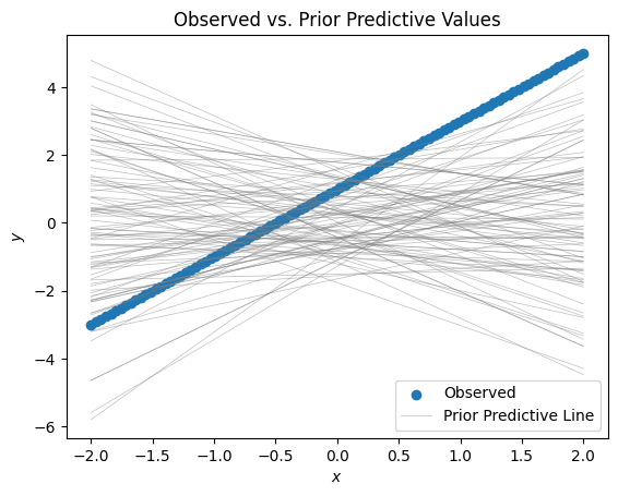

A plot of the priors against the model, showing a very poor fit

As you can see, this is ridiculous - our priors don’t even come close to capturing the spirit of the data.

Now, we should be careful here. After all, we don’t really want our priors to exactly capture the data - one of the strengths of the Bayesian way of doing inference is that it accounts for uncertainty. If we really wanted to, we could just apply the formulat for a least-squares regression line, but we want to give our model some flexibility.

If this were a real-world situation, we might consult some experts and see what sort of ranges they would consider reasonable or make use of physical constraints to help mold our priors. However, since this is a contrived situation we can also be a bit contrived in how we tighten our priors up.

Let’s say that we have solicited some expert opinions or whatnot, and they are all unanimous that the intercept for the line should be between about 0 and 2 and the slope should be between 1 and 3. Since we are using normal priors, let’s fix it so that at least initially, the means are the midpoints of the ranges and about 95% ( $\sim 2 \sigma$ ) of the mass of the function is in the specified range.

b0_range = np.array([ 0, 2 ])
b1_range = np.array([ 1, 3 ])
with pm.Model() as model:
    sigma = pm.Exponential('sigma', 1)
    b0 = pm.Normal('b0', b0_range.mean(), 1/2)
    b1 = pm.Normal('b1', b1_range.mean(), 1/2)
    mu = b0 + b1 * x
    y = pm.Normal('y', mu=mu, sigma=sigma, observed=observed_y)
    prior = pm.sample_prior_predictive(samples=1000)

fig, ax = plt.subplots()
ax.scatter(x, true_y, label="Observed")
for sample_num in range(100):
    index = np.random.randint(0, 500 + 1)
    sample_m = prior['b0'][index]
    sample_b = prior['b1'][index]
    sample_y = sample_m * x + sample_b
    ax.plot(x, sample_y, color='grey', linewidth=0.5, alpha=0.5, label="Prior Predictive Line" if sample_num == 0 else None)
ax.set_xlabel('$x$')
ax.set_ylabel('$y$')
ax.set_title('Observed vs. Prior Predictive Values (Better Priors)')
ax.legend()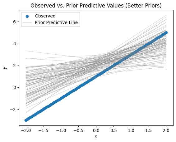

A plot of the posterior against the observed data, showing a somewhat better fit

This seems much more credible. Of course, it doesn’t quite look like our data, but that’s where the fitting step comes in.

Fitting the Model

So far we’ve created the model, but we haven’t actually used any of the observed data! At this point that’s easy - we can sample from the posterior.

with model:
    trace = pm.sample(draws=1000)

  return wrapped_(*args_, **kwargs_)
Auto-assigning NUTS sampler...
Initializing NUTS using jitter+adapt_diag...
Multiprocess sampling (4 chains in 4 jobs)
NUTS: [b1, b0, sigma]

100.00% [8000/8000 00:01<00:00 Sampling 4 chains, 0 divergences]

Sampling 4 chains for 1_000 tune and 1_000 draw iterations (4_000 + 4_000 draws total) took 1 seconds.

Now we should take a look at our data. PyMC has a traceplot funtion to see the results, and the arViz package can be used as well. Let’s see what that looks like!

pm.traceplot(trace)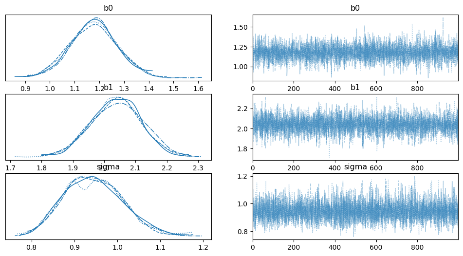

A plot of the posterior distributions of the model parameters

az.plot_posterior(trace)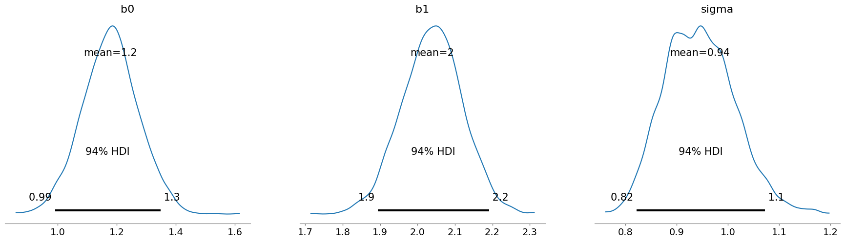

A plot of the posterior distribution of the model parameters

From these, we can see that the posteriors seems reasonable. With the benefit of knowing the actual true values, we can see that they fall right in the right range. However, we would really like to be a bit more sure. For that, we will use the posterior to generate some predictions.

Checking the Model

To check the model, we would like to have it make some predictions (against the data that we used to train it) and then see how that stacks up against what we actually have. This is really the lowest bar that a model should be able to clear - retrodicting the data that was used to train it! Unfortunately, at the moment there’s not a good way to do that. Instead, we need to modify the model a bit to allow us to generate some predictions.

with pm.Model() as model:
    sigma = pm.Exponential('sigma', 1)
    b0 = pm.Normal('b0', b0_range.mean(), 1/2)
    b1 = pm.Normal('b1', b1_range.mean(), 1/2)
    # this is what we changed - we'll reach back in later and change this to produce a prediction
    data = pm.Data('x', x)
    mu = b0 + b1 * data
    y = pm.Normal('y', mu=mu, sigma=sigma, observed=observed_y)
    trace = pm.sample()

  return wrapped_(*args_, **kwargs_)
Auto-assigning NUTS sampler...
Initializing NUTS using jitter+adapt_diag...
Multiprocess sampling (4 chains in 4 jobs)
NUTS: [b1, b0, sigma]

100.00% [8000/8000 00:01<00:00 Sampling 4 chains, 0 divergences]

Sampling 4 chains for 1_000 tune and 1_000 draw iterations (4_000 + 4_000 draws total) took 1 seconds.

new_xs = np.array([-2, 0, 2])
with model:
    pm.set_data({'x': new_xs})
    posterior = pm.sample_posterior_predictive(trace)
posterior

100.00% [4000/4000 00:03<00:00]

{'y': array([[-4.31035799,  1.57566098,  5.42077205],
        [-1.55553502,  2.03654546,  7.24123784],
        [-3.9617322 , -0.25304165,  4.33324207],
        ...,
        [-4.37924564,  0.93889857,  5.34962462],
        [-2.14268032,  2.04171249,  5.84599946],
        [-2.90813163,  1.25685193,  4.94745574]])}

posterior['y'].shape

(4000, 3)

The variable posterior is a dict with a single key, y, which contains the different samples for y at the different values of x. That is, posterior['y'] is an array of 4000 arrays, each of length three, representing a sample of y at the values of x we specified: new_xs. This then allows us to plot the values that we got back!

predicted = posterior['y']

# these are each arrays of length three, representing the mean
# and std of the y values at each of the prediction x values
y_mean = predicted.mean(axis=0)
y_std = predicted.std(axis=0)

fig, ax = plt.subplots()
ax.scatter(x, true_y, label="Observerd Data", alpha=0.5)
ax.plot(new_xs, y_mean, label="Predicted mean value")
ax.fill_between(new_xs, y_mean - 2 * y_std, y_mean + 2 * y_std, label="$\mu \pm 2 \sigma$", alpha=0.2)

ax.legend()
ax.set_xlabel("$x$")
ax.set_ylabel("$y$")
ax.set_title("Comparison of Observed Data and Posterior Prediction")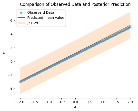

A plot showing a good fit between the posterior predictions and the observed data

From this, we can see that there is a good fit between our posterior and observed data.

Conclusion

So there we have it! This has been a short trip through a simple Bayesian workflow, highlighting some of the steps and validation that we should do as we build and fit a model. Hopefully this has given you an idea of how you can use PyMC to work on your pwn statistical problems.