Confidence Intervals of a Difference of Means With Large Sample Sizes
Finding a confidence interval for different population means when we can take large sample sizes
As part of my plan to correct my sadly lacking education in statistics, I have been looking into figuring out differences in population means! It turns out that there’s a lot more to this than I initially though, so I’ve decided to break the idea up into a few different areas. The first is the easiest - figuring out how different two populations are when we can take large samples of both.
One of the things that we might want to do when investigating the differences between two populations is to find out how different their means could be; this is, we would like to create a confidence interval for the difference between the two means.
For now, let’s assume that we have two populations, and the quality that we’re measuring is normally distributed (height, maybe). For the first population, the height has mean and variance , and for the second and . We’re interested in the differences in height between the two populations. We start by drawing a sample of size from the first population and another of size from the second. Since the two populations are normally distributed, so is the parameter of interest, . To see why, let’s take a look at the sample means.
Each sample mean, and , has a sampling distribution of . We know that if you have two different normal variables, say
then their sum is
Similarly, if you have a constant multiple of a normally distributed variable, the resulting variable is also normally distributed:
Thus, their difference has a sampling distribution of
Given that it’s normally distributed, we can calculate the statistic; that is, if we set the significant level to , then with probability , the variable
will lie between and . (Note that this is just the regular definition of but with the values for the difference of means subbed in). We can use this fact to find the confidence interval for the true difference by isolating :
Or to put it another way, the confidence interval for the difference in means is
An example
Let’s say you’re comparing chemistry test scores between two different schools. School A has 50 students taking the test and School B has 75. School A has an average grade of 76 with a standard deviation of 6, while School B has an average grade of 82 with a standard deviation of 8. What is the 96% confidence interval for the difference in their test scores?
(Adapted from Walpole & Myers (1985), example 7.6, p. 227)
Luckily, this question has all of the information we need to compute the answer simply by plugging in to the above formula.
# School A
x_bar_1 <- 76
s_1 <- 6
n_1 <- 50

# School A
x_bar_2 <- 82
s_2 <- 8
n_2 <- 75

# significance level
alpha <- 1 - 0.97

mean_estimate <- x_bar_1 - x_bar_2 # -6
critical_value <- qnorm(alpha / 2, lower.tail = FALSE) # 2.05
sample_sd <- sqrt(( s_1 ^ 2 ) / n_1 + ( s_2 ^ 2 ) / n_2) # 1.25
(ci <- mean_estimate + c(-1, 1) * critical_value * sample_sd)- -8.57607034421222
- -3.42392965578778
So the 96% confidence interval for the difference is about ; we can say that we are 96% confident that the scores for School A are 8.57% - 3.42% lower than those for School B.
We can also interpret this graphically:
library(ggplot2)

add_annotated_arrow <- function(p, start, end, text=NA, text_shift=c(0,0)) {
    p <- p +
    geom_segment(aes(x=start[1], y=start[2], xend=end[1], yend=end[2]), arrow=arrow())

    if (!is.na(text)) {
        p <- p + annotate('text', x=start[1] + text_shift[1], y=start[2] + text_shift[2], label=text)
    }
    return(p)
}

NUM_SDS = 4
x <- seq(from=mean_estimate - NUM_SDS * sample_sd, to=mean_estimate + NUM_SDS * sample_sd, length.out=1001)
plot_df <- data.frame(x=x, score_distribution=dnorm(x, mean=mean_estimate, sd=sample_sd))

p <- ggplot(plot_df, aes(x, score_distribution)) +
    geom_line() +
    # shade in the confidence interval
    geom_ribbon(data=subset(plot_df, x >= ci[1] & x <= ci[2]), aes(ymax=score_distribution), ymin=0, fill='blue', colour=NA, alpha=0.5) +
    # emphasize the critical values
    geom_segment(aes(x=ci[1], y=0, xend=ci[1], yend=dnorm(ci[1], mean=mean_estimate, sd=sample_sd))) +
    geom_segment(aes(x=ci[2], y=0, xend=ci[2], yend=dnorm(ci[2], mean=mean_estimate, sd=sample_sd))) +
    # set the ticks
    scale_x_continuous(breaks=c(-9, ci[1], -6, ci[2], -3), labels=c("-9", round(ci[1], 2), "-6", round(ci[2], 2), "-3")) +
    # titles, &c.
    ggtitle("Distribution for the difference in scores") +
    xlab("Difference in Scores") +
    ylab("Probability Density")

# add in arrows and annotations
# critical points
p <- add_annotated_arrow(p, start=c(-2, 0.15), end=c(ci[1] + 0.1, dnorm(ci[1], mean=mean_estimate, sd=sample_sd)))
p <- add_annotated_arrow(p, start=c(-2, 0.15), end=c(ci[2] + 0.1, dnorm(ci[2], mean=mean_estimate, sd=sample_sd)), text="Critical Points", text_shift=c(0, 0.01))
# confidence region
p <- add_annotated_arrow(p, start=c(-3, 0.2), end=c(-6, 0.15), text="96% Confidence Region", text_shift=c(0, 0.01))
ggsave("96ci.jpg", dpi=300)
print(p)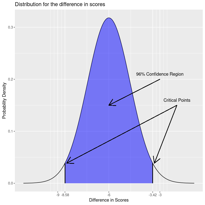
And there we have it - a way to calculate the confidence for the means of two populations when we are able to draw a large sample. The next obvious step is to deal with the case where we can’t draw a large sample. It turns out that this is substantially more complicated, and so will be left for later!
Sources
- Bevans, R. (2023, June 22). An Introduction to t Tests | Definitions, Formula and Examples. Scribbr. https://www.scribbr.com/statistics/t-test/
- Walpole, R. E., & Myers, R. H. (1985). Probability and Statistics for Engineers and Scientists. Macmillan USA.
- Sampling distribution. (2023). In Wikipedia. https://en.wikipedia.org/w/index.php?title=Sampling_distribution&oldid=1181679769