Sampling Distributions for the Mean and Standard Deviation
Quick introduction to some sampling distribution for the mean / standard deviation, introducing the Central Limit Theorem and the Student t distribution.
This post is a continuation of the previous one on confidence intervals for the mean with large sample sizes.
Before we continue on with our exploration of confidence intervals, we should talk more about what exactly a sampling distribution is. Imagine that we have some sort of property of a group that we’re interested in (say, the height). This property has some sort of underlying distribution which we want to know about. However, generally we can’t find this exactly; that would be far too costly in terms of both time and money. So instead, we take samples from the population and use that to reason about the underlying distribution. For instance, in our example, if we want to know something about the distribution of heights, we might take a group of people, measure their heights, take the mean, and use that as a proxy for the mean of the heights in the population.
However, that measurement, the mean of a sample, will not always be the same. If we run the experiment 100 times, and each time take a group of 10 people and measure their heights, we won’t always get the same mean. Instead, the mean we measure will have its own distribution, separate from but related to the underlying distribution of heights! The distribution of measurements that we derive from the sample is a sample distriution - the probability distribution for some statistic that we calculate from a sample.
There are all kinds of different measurements that we might want to calculate from a sample - mean, standard deviation, range, &c. - but here we’ll focus on the two most common: the mean and ones related to the standard deviation.
Means
Let’s start with the sampling distribution for the mean. Imagine that we are drawing samples from a normal distribution . Since each observation comes from a normal distribution, it is distributed normally. Hence,
Since by the properties of the normal distribution, the mean of a sum of normals is the sum of their means
and the variance is the sum of the variances:
Note that the standard error for some statistic is the standard deviation of its sampling distribution. In this case (the mean), that is .
Let’s see this in action!
The heights in a population are normally distributed with a mean of 176cm and a standard deviation of 6cm. If we are taking samples of 10 people and finding their mean heights, what is the distribution that we expect to see?
Here we have all the the information that we need - namely, the population mean, standard deviation, and size of the sample. Thus, we expect that sample means to be distributed as
Let’s see if this actually matches with a simulation.
NUM_SAMPLES <- 1000

n <- 10
mu <- 176
sd <- 6

# generate the sets of samples from the population (result is a matrix where the columns are the samples)
height_samples <- replicate(NUM_SAMPLES, rnorm(n, mean=mu, sd=sd))
# now calculate the mean (margin 2 means the columns)
simulated_means <- apply(height_samples, 2, mean)
# Plotting the results
library(ggplot2)
NUM_SDs <- 3
heights <- seq(from=mu-NUM_SDs/sqrt(n) *sd, to=mu+NUM_SDs/sqrt(n)*sd, by=0.1)
# first the predicted, then the actual
predicted_df <- data.frame(
heights=heights,
density=dnorm(heights, mean=mu, sd=sd / sqrt(n)),
type="Predicted N(176, 6 / sqrt(10))"
)
simulated_df <- data.frame(
heights=simulated_means,
type="Simulated"
)
p <- ggplot(simulated_df, aes(heights)) +
geom_histogram(binwidth = 1, mapping=aes(y=after_stat(density), color=type)) +
geom_line(data=predicted_df, aes(x=heights, y=density, color=type), linewidth=2) +
scale_colour_grey() +
xlab("Height") +
ylab("Density") +
ggtitle("Predicted and Simulated Sample Means (n=10)")
print(p)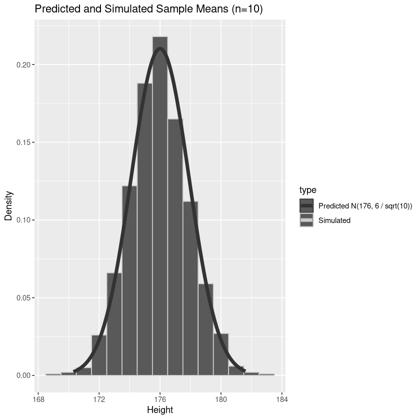
From this plot, we can see that the empirical distribution of the sample means is in excellent agreement with our predicted distribution.
Central Limit Theorem
It gets better! Above, we assumed that the distribution from which we were drawing was normal. However, it turns out that this same approach works with any distribution with a finite mean and finite variance :
Central Limit Theorem: If is the mean of a sample of size from a distribution with mean and finite variance , then the score
in the limit is distributed as .
Let’s see this in action!
NUM_SAMPLES <- 1e4
NUM_SDs <- 3
x <- seq(-NUM_SDs, NUM_SDs, by=0.1)
y <- dnorm(x, mean=0, sd=1)
simulated <- data.frame(x=x, means=y)

# Uniform distribution
a <- 0
b <- 1
mu <- (a + b) / 2
sigma <- sqrt((a - b)^2 / 12)

unif_means <- apply(replicate(NUM_SAMPLES, runif(10, 0, 1)), 2, mean)
# standardize
unif_means <- (unif_means - mu) / (sigma / sqrt(n))

empirical <- data.frame(x=unif_means)

p <- ggplot(simulated, aes(x)) +
    # what we actually got
    geom_histogram(data=empirical, aes(y=after_stat(density)), binwidth=0.1) +
    # what the distribution should approach
    geom_line(aes(y=means), linewidth=2)
print(p)
# binomial distribution
binomial_n <- 100
p <- 0.5
mu <- binomial_n * p
variance <- binomial_n * p * (1 - p)
sigma <- sqrt(variance)

binomial_means <- apply(replicate(NUM_SAMPLES, rbinom(n, binomial_n, p)), 2, mean)
# standardize
binomial_means <- (binomial_means - mu) / (sigma / sqrt(n))
empirical <- data.frame(x=binomial_means)

p <- ggplot(simulated, aes(x)) +
    # what we actually got
    geom_histogram(data=empirical, aes(y=after_stat(density)), bins=40) +
    # what the distribution should approach
    geom_line(aes(y=means), linewidth=2)
print(p)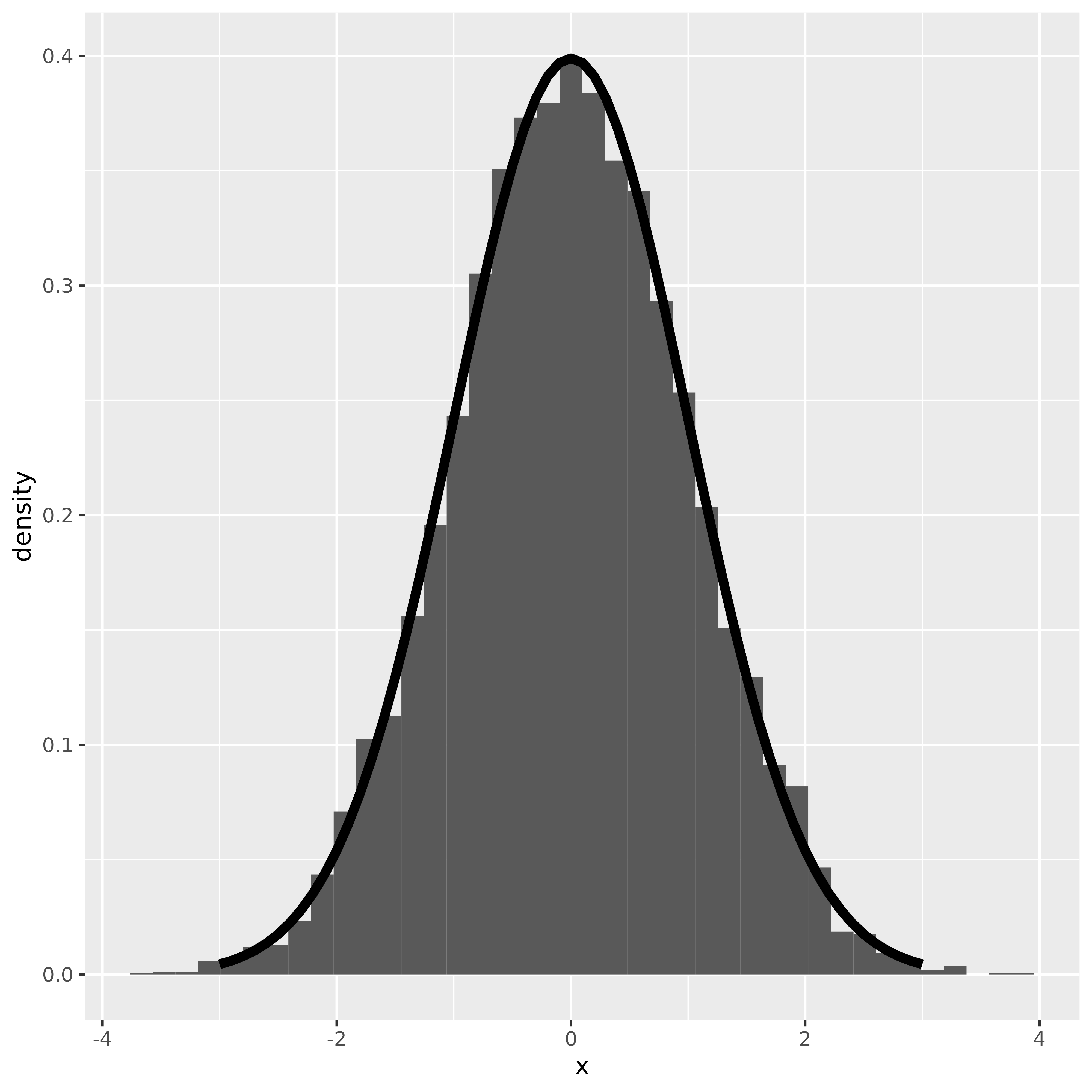
And once again, we see that there is good agreement between the predicted standard normal and the standardized sample mean. The Central Limit Theorem is very handy because it means that as long as the basic distribution from which we’re sampling from is reasonably well behaved, then the standardized means will have the same sampling distribution - .
Sampling Distributions Related to the Variance
In addition to the mean, we can also consider the sampling distribution of the sample variance, . In practice, we rarely care about this directly. However, it can be useful to consider it in the context of other problems. In particular, note that to use the CLT above we needed to know both the mean and variance of the underlying distribution. In the absence of other data, the sample mean is a good proxy for the distribution mean, even for relatively small sample sizes. However, the sample variance can vary widely and is often not a great representation of the underlying variance.
To start with, let’s consider the sampling distribution, not of , but of the related quantity (for reasons that will become clear later). To start:
Dividing each side by , substituting in , and rearranging for our term of interest,
I’m now going to assert a few things entirely without proof.
- Expression 1 is distributed as a chi-squared distribution with degrees of freedom
- Epression 2 is the square of a normally distributed variable (in fact, we looked at this just above!), and thus is distributed as chi-squared distribution with one degree of freedom
- is distributed as a chi-squared distribution with degrees of freedom
Distribution
To use the CLT, we need to calculate the sample statistic
However, we generally don’t know the sample standard deviation , and so we substitute in the sample variance instead to get the related, evocatively named, statistic
If we have large sample sizes, then the value of is close to and so this is still distributed as a standard normal. However, if we have small sample sizes than varies more than we would expect, and so the resulting distribution is not normal.
We can rewrite this slightly by dividing both the numerator and denominator by :
where
and
We know that is distributed as a standard normal, and from what we learnt earlier is chi-squared with degrees of freedom. Their quotient, , is distributed as a distribution with degrees of freedom. The distribution (also called the Student’s distribution) is a lot like the normal distribution, but has much fatter tails. In practice, this means that extreme events (far from the mean) are unlikely bordering on impossible in the normal, but are far more likely (less surprising) with the distribution. As the number of degrees of freedom () increases, the distribution aproaches the normal, as we would expect.
library(ggplot2)

x <- seq(-4, 4, by=0.1)
df_1 <- dt(x, 1)
df_2 <- dt(x, 2)
df_5 <- dt(x, 5)
df_inf <- dt(x, Inf)

plot_df <- data.frame(
    x=rep(x, 4),
    y=c(df_1, df_2, df_5, df_inf),
    df=rep(c(1, 2, 5, Inf), each=length(x))
)

ggplot(plot_df, aes(x, y, group=df)) +
    geom_line(aes(colour=df), linewidth=2) +
    labs(title="Student t Distribution", x="x", y="Density", colour="Degrees of Freedom")
ggsave("student_t.png", dpi=600)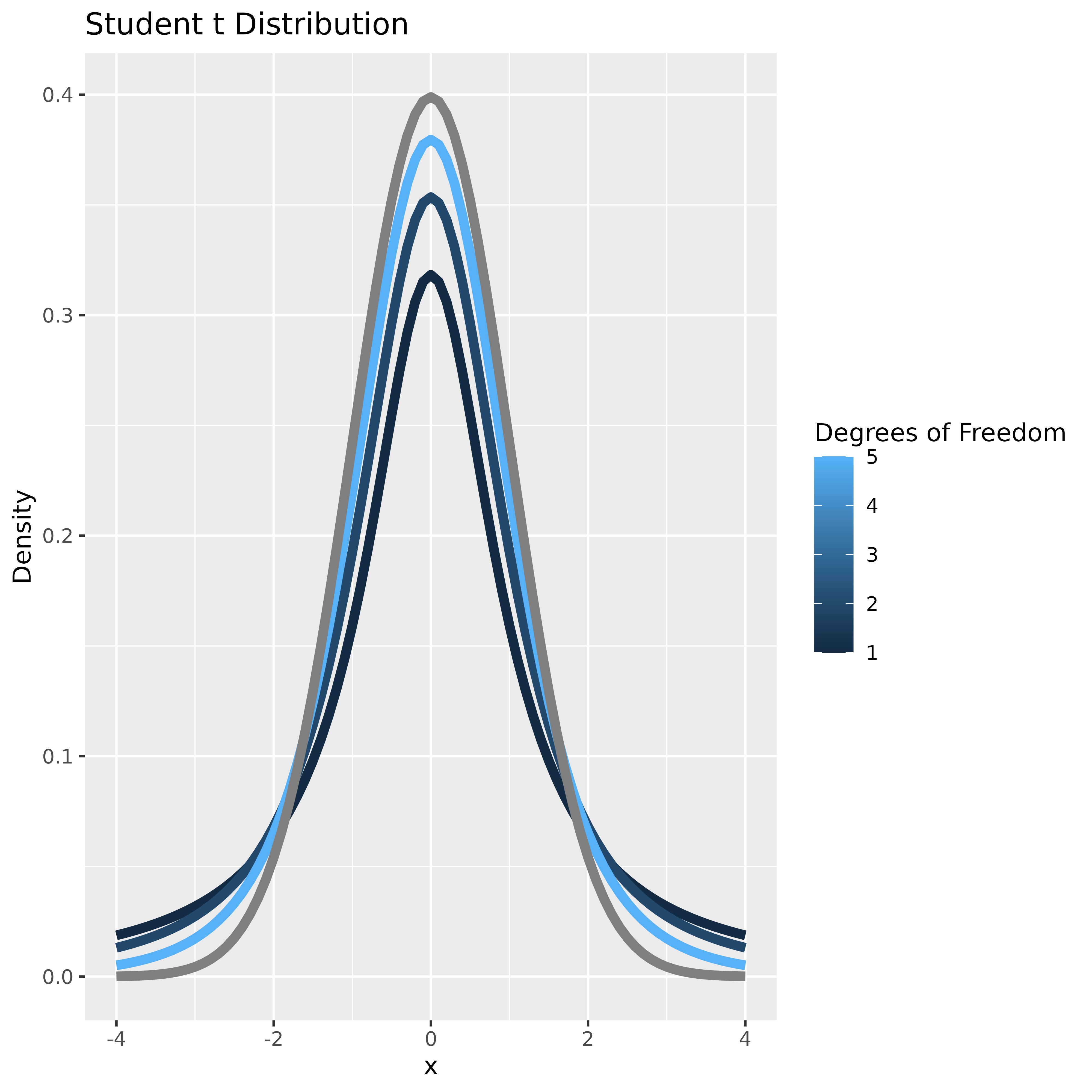
Summary
Today’s post was very much an interstitial one. We looked at some sampling distributions for means and variances (kind of), introducing the central limit theorem and the Student distribution along the way. Next time, we’ll see how we can use these facts to derive confidence intervals for a difference in means using small sample sizes!
Sources
- Chi-squared distribution. (2023). In Wikipedia. https://en.wikipedia.org/w/index.php?title=Chi-squared_distribution&oldid=1186546774
- Sampling distribution. (2023). In Wikipedia. https://en.wikipedia.org/w/index.php?title=Sampling_distribution&oldid=1181679769j
- Standard error. (2023). In Wikipedia. https://en.wikipedia.org/w/index.php?title=Standard_error&oldid=1183182476
- Student’s t-distribution. (2023). In Wikipedia. https://en.wikipedia.org/w/index.php?title=Student%27s_t-distribution&oldid=1179322277
- Walpole, R. E., & Myers, R. H. (1985). Probability and Statistics for Engineers and Scientists. Macmillan USA.