Exploring Population Differences Using Bayesian Analysis In R with RStan
This post is concerned with the eventual goal of exploring population differences (e.g. differences in means) using Bayesian analysing using Stan and RStan, the R interface to Stan.
Continuing on with the theme of modelling population differences, this post will examine that process using the popular Bayesian language / platform, Stan.
The first step will be to install RStan. This is an interface between Stan and R, allowing you to run Stan models from within R. This process is notoriously fiddly and difficult, but the instructions on the RStan page are very good and as long as you follow the steps you should be fine.
First, let’s load the package.
library(rstan)

# recommended options
options(mc.cores = parallel::detectCores())
rstan_options(auto_write = TRUE)
rstan_options(threads_per_chain = 1)

packageVersion("rstan")
[1] ‘2.32.3’The first thing that we’ll do is run a very simple model: recovering the parameters for a Gaussian from a random selection from the distribution.
NUM_SAMPLES <- 1e3
mu <- 0
sigma <- 1

w <- rnorm(NUM_SAMPLES, mean=mu, sd=sigma)
Now that we have the data, we need to write the model in Stan. The format is very similar to the way that we wrote the model above. The code for the above model looks like the below in Stan.
// simple_model.stan

// this section is the data that we will add to the model
data {
    int<lower=0> n; // number of samples
    vector[n] w; // the actual samples
}

// these are the parameters to be used in the model
parameters {
    real mu;
    real<lower=0> sigma;
}

// the actual model
model {
    mu ~ normal(0, 1);
    sigma ~ normal(0, 1);

    w ~ normal(mu, sigma); // this describes how the data are distributed
}
Note that in order to avoid an error saying something about an incomplete line, just add a blank line to the end of the Stan file. Apparently it’s a known issue.
Now let’s fit the model using the stan, get a summary, and then extract the parameters (as samples). We need to specify the file which contains the Stan models, along with the data (formatted as a list).
data <- list(n=length(w), w=w)
fit <- stan(file='simple_model.stan', data=data)
summary(fit)- $summary
A matrix: 3 × 10 of type dbl mean se_mean sd 2.5% 25% 50% 75% 97.5% n_eff Rhat mu 0.02597236 0.0005827845 0.03262796 -0.04121622 4.538632e-03 0.0260687 0.04786533 0.09049842 3134.468 1.000547 sigma 1.01445024 0.0004267207 0.02287461 0.97043331 9.984133e-01 1.0143704 1.03004736 1.05924737 2873.557 1.001364 lp__ -515.24968715 0.0258127557 1.02424096 -518.00629800 -5.156437e+02 -514.9284938 -514.51819964 -514.24947892 1574.474 1.001698 - $c_summary
Looking at the mean for our parameters, it looks like our model did a good job of recovering the values. Let’s take a mode detailed look by extracting some samples.
params <- extract(fit)
summary(params)
Length Class Mode
mu 4000 -none- numeric
sigma 4000 -none- numeric
lp__ 4000 -none- numericThis contains the different samples for the parameters. With the benefit of knowing the underlying distribution, we can plot some of these to see how well we did.
library(ggplot2)
options(repr.plot.width=15, repr.plot.height=8)
x <- seq(-4, 4, by=0.1);
true <- dnorm(x, 0, 1)
plt <- ggplot(data.frame(x=x, y=true), aes(x, y)) +
geom_line(colour='black', linewidth=2) +
labs(x='w', y='Density', title="Simulated data for the mean")
for (index in sample(1:nrow(params$mu), 20, replace = TRUE)) {
df <- data.frame(x=x, y=dnorm(x, mean=params$mu[index]), sd=params$sigma[index])
plt <- plt +
geom_line(data=df, mapping=aes(x, y), colour='blue', alpha=0.2)
}
print(plt)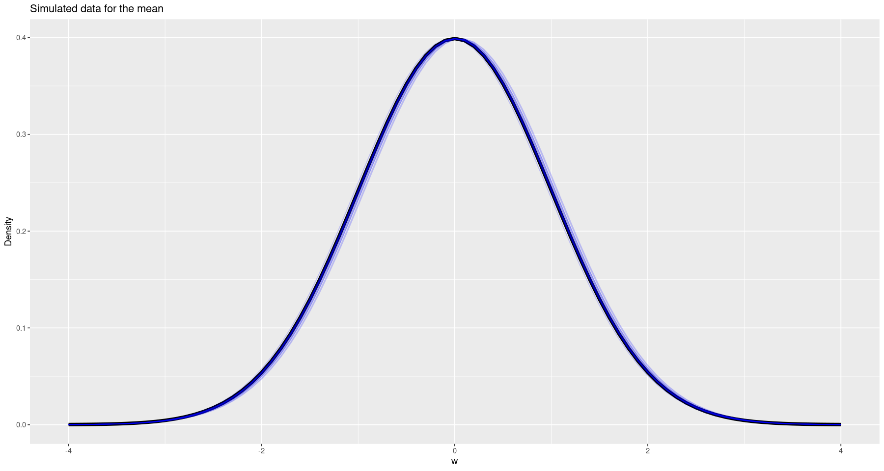
So this looks pretty good!
Of course, we could do better by doing a posterior predictive check - that is, using our final model to generate some data to ensure that it looks like the data that was used to fit the model. To do this, we can actually add some predicted data into the model. We just need to make a small modification to the Stan model.
// simple_model_ppc.stan

// this section is the data that we will add to the model
data {
    int<lower=0> n; // number of samples
    vector[n] w; // the actual samples
}

// these are the parameters to be used in the model
parameters {
    real mu;
    real<lower=0> sigma;
}

// the actual model
model {
    mu ~ normal(0, 1);
    sigma ~ normal(0, 1);

    w ~ normal(mu, sigma); // this describes how the data are distributed
}

// this is the section that we change - we want to add a posterior predictive check
generated quantities {
    vector[n] w_sim;

    for (i in 1:n) {
        w_sim[i] = normal_rng(mu, sigma);
    }
}
ppc_fit <- stan(file="simple_model_ppc.stan", data=data)
summary(ppc_fit)
ppc_params <- extract(ppc_fit)- $summary
A matrix: 1003 × 10 of type dbl mean se_mean sd 2.5% 25% 50% 75% 97.5% n_eff Rhat mu 0.025810450 0.0005388202 0.03148880 -0.03338427 0.004332818 0.025322161 0.04692252 0.08776891 3415.266 1.0005321 sigma 1.015913201 0.0003754666 0.02276205 0.97354499 0.999955002 1.015059556 1.03107722 1.06183558 3675.192 0.9999481 w_sim[1] 0.012561131 0.0161172391 1.02058732 -2.01894175 -0.657810006 0.007209496 0.69260442 1.97101691 4009.766 0.9996054 w_sim[2] 0.040253027 0.0161314894 1.01840079 -1.91445011 -0.656381401 0.030597371 0.73512073 2.01208962 3985.552 0.9995883 w_sim[3] 0.022706146 0.0160527865 1.01124083 -1.95816825 -0.651363176 0.044916355 0.71121470 1.96146212 3968.335 1.0006904 w_sim[28] 0.033896862 0.0172899348 1.01121499 -2.00957414 -0.629203502 0.035372024 0.70714091 1.99001365 3420.584 1.0002338 ⋮ ⋮ ⋮ ⋮ ⋮ ⋮ ⋮ ⋮ ⋮ ⋮ ⋮ w_sim[972] 5.552801e-02 0.01623083 1.0229120 -1.983298 -0.6182711 5.770454e-02 0.7213428 2.055063 3971.872 0.9997000 w_sim[1000] 4.159035e-02 0.01720112 1.0235276 -2.003147 -0.6280401 6.721470e-02 0.7225033 2.064001 3540.670 0.9998228 lp__ -5.152061e+02 0.02251679 0.9588736 -517.805703 -515.5911481 -5.149248e+02 -514.5125150 -514.251023 1813.467 1.0002974 - $c_summary
Now we can compare our data to the simulated results by choosing 10 random bunches of simulated data and graphing it, along with the actual data.
df <- data.frame(w=w)

plt <- ggplot(df, aes(w)) +
    geom_density(aes(y=after_stat(scaled)), linewidth=2, colour='black') +
    labs(x='w', y="Density", title="Comparison of actual vs. simulated data")


for(index in sample(1:nrow(ppc_params$w_sim), 10)) {
    plt <- plt +
        geom_density(data=data.frame(x=ppc_params$w_sim[index,]), mapping=aes(x, y=after_stat(scaled)), colour=alpha('blue', 0.2))
}
print(plt)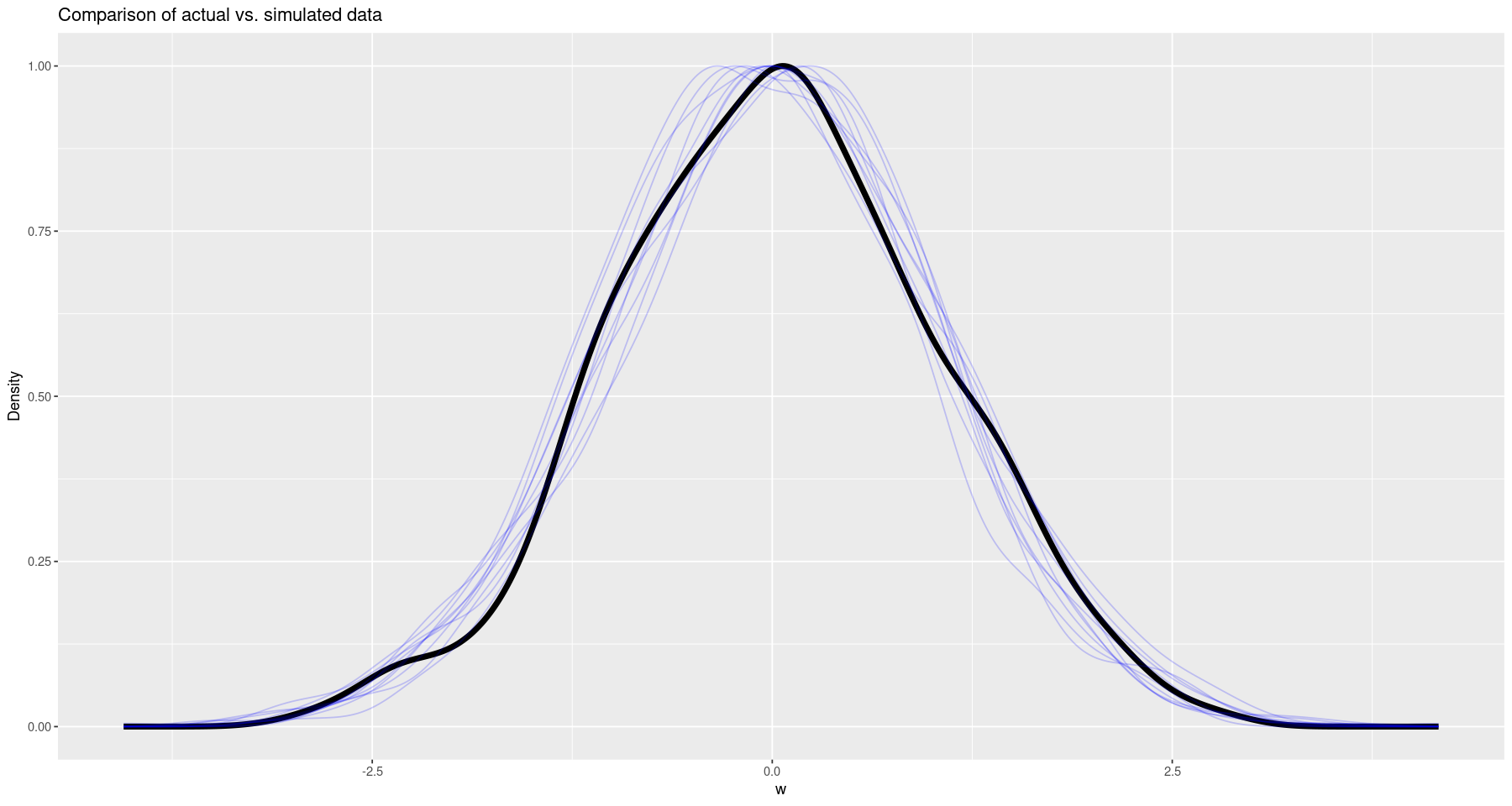
Using Summary Statistics
In addition to using the actual data, we can also use the summary statistics (sample mean and sample standard deviation) to generate a posterior. I’ve found this to be useful in the case where the raw data is inaccessible (due to age or other restrictions) but the summary statistics have been published. To do this, we rely on two facts:
Both of these facts can be encode in a Stan model.
// simple_model_ppc_summary.stan

// this section is the data that we will add to the model
data {
    int<lower=0> n; // number of samples
    real x_bar; // sample mean
    real<lower=0> s; // sample standard deviation
}

// these are the parameters to be used in the model
parameters {
    real mu;
    real<lower=0> sigma;
}

// the actual model
model {
    mu ~ normal(0, 1);
    sigma ~ normal(0, 1);

    real modified_s = (n - 1) * s^2 / sigma^2;

    x_bar ~ normal(mu, sigma / sqrt(n)); // this describes how the data are distributed
    modified_s ~ chi_square(n - 1);
}

// data for the posterior predictive check
generated quantities {
    vector[n] w_sim;

    for (i in 1:n) {
        w_sim[i] = normal_rng(mu, sigma);
    }
}
summary_fit <- stan(file='simple_model_ppc_summary.stan', data=list(n=length(w), x_bar=mean(w), s=sd(w)))
summary(summary_fit)- $summary
A matrix: 1003 × 10 of type dbl mean se_mean sd 2.5% 25% 50% 75% 97.5% n_eff Rhat mu 0.024834235 0.0005916098 0.03339289 -0.03943811 0.002238256 0.024639415 0.04706407 0.09141525 3185.937 1.0013604 sigma 1.015434182 0.0004143965 0.02306986 0.97260845 0.999503487 1.014924975 1.03053549 1.06160283 3099.258 1.0000964 w_sim[1] 0.014455045 0.0159013104 1.01510507 -1.91725272 -0.690326722 0.018145823 0.69572528 2.00411045 4075.268 1.0010727 w_sim[28] 0.042364698 0.0157351743 0.99763643 -1.93211158 -0.630438791 0.046843407 0.72574547 1.97958825 4019.773 1.0014029 ⋮ ⋮ ⋮ ⋮ ⋮ ⋮ ⋮ ⋮ ⋮ ⋮ ⋮ w_sim[972] 1.024258e-02 0.01653087 1.0225007 -2.018235 -0.6773512 2.487396e-02 0.7090567 1.980203 3825.918 1.0001160 w_sim[1000] -5.485209e-03 0.01707601 1.0254360 -2.008587 -0.6838811 -2.336391e-04 0.6810644 2.015877 3606.153 1.0010102 lp__ 2.945402e+03 0.02635960 1.0639737 2942.602144 2944.9820042 2.945726e+03 2946.1466281 2946.430291 1629.237 1.0020386 - $c_summary
summary_params <- extract(summary_fit)Once again, we can visually check against the original data.
df <- data.frame(w=w)

plt <- ggplot(df, aes(w)) +
    geom_density(aes(y=after_stat(scaled)), linewidth=2, colour='black') +
    labs(x='w', y="Density", title="Comparison of actual vs. simulated data (from summary data)")


for(index in sample(1:nrow(summary_params$w_sim), 10)) {
    plt <- plt +
        geom_density(data=data.frame(x=summary_params$w_sim[index,]), mapping=aes(x, y=after_stat(scaled)), colour=alpha('blue', 0.2))
}
print(plt)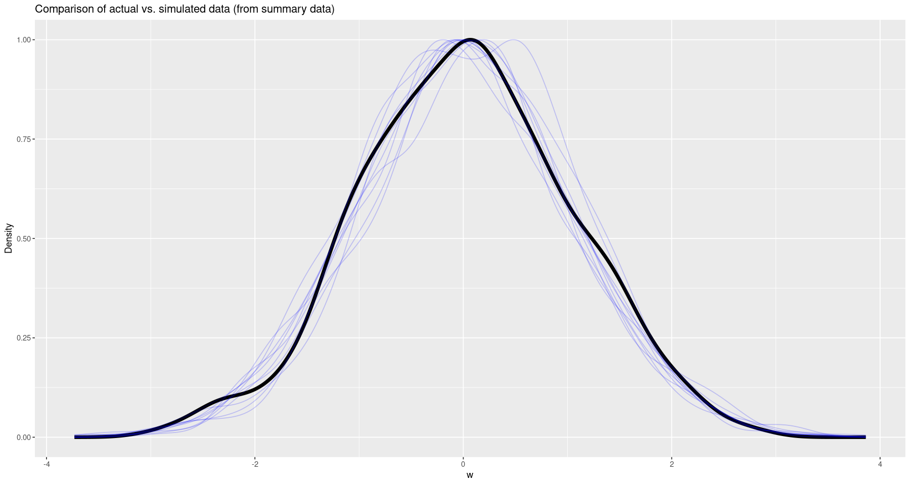
Difference of Means
Now that we have the basics out of the way, we can look at the distribution of the differences in means between two populations! The first method we’ll use is to model each population separately, and then get the distribution of the difference of means from that.
data {
    int<lower=0> N;
    vector[N] w_1;
    vector[N] w_2;
}

parameters {
    real mu_1;
    real mu_2;
    real<lower=0> sigma;
}

model {
    mu_1 ~ normal(0, 2);
    mu_2 ~ normal(0, 2);
    sigma ~ normal(0, 1);

    w_1 ~ normal(mu_1, sigma);
    w_2 ~ normal(mu_2, sigma);
}
mu <-c(-1, 1)
sigma <- 1

w_1 <- rnorm(NUM_SAMPLES, mean=mu[1], sd=sigma)
w_2 <- rnorm(NUM_SAMPLES, mean=mu[2], sd=sigma)

difference_fit <- stan(file='difference_means.stan', data=list(N=NUM_SAMPLES, w_1=w_1, w_2=w_2))
summary(difference_fit)- $summary
A matrix: 4 × 10 of type dbl mean se_mean sd 2.5% 25% 50% 75% 97.5% n_eff Rhat mu_1 -1.0106497 0.0004784863 0.03100593 -1.0720868 -1.0305666 -1.0105328 -0.9895498 -0.9509228 4199.043 0.9995809 mu_2 0.9976796 0.0004909118 0.03090297 0.9376764 0.9767728 0.9977505 1.0185254 1.0587181 3962.721 0.9996719 sigma 0.9820112 0.0002207197 0.01584171 0.9512097 0.9714469 0.9818158 0.9922650 1.0131478 5151.362 1.0000500 lp__ -964.0037707 0.0275646936 1.26107968 -967.1965946 -964.5648992 -963.6988244 -963.0975006 -962.5887301 2093.046 1.0043513 - $c_summary
difference_params <- extract(difference_fit)
differences <- difference_params$mu_1 - difference_params$mu_2

ggplot(data.frame(x=differences), aes(x)) +
    geom_density(aes(y=after_stat(scaled))) +
    labs(x="Difference", y="Density", title="Distribution of the Difference")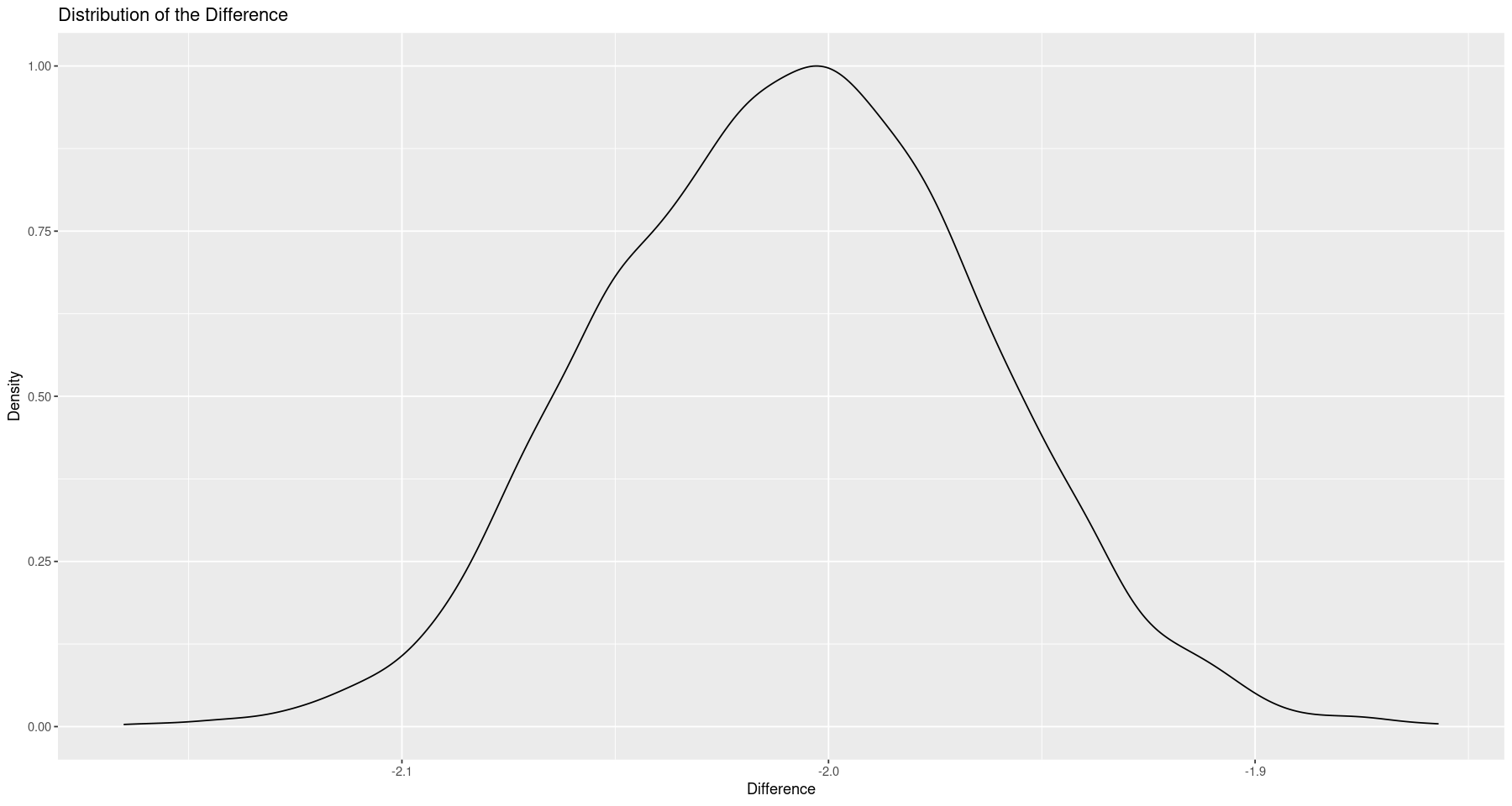
This is basically what we expected to see - a difference of 2. If we wanted, we could also extract a credible interval from the data.
diff_ci <- quantile(differences, probs=c(0.025, 0.975))
diff_ci- 2.5%
- -2.09156770868759
- 97.5%
- -1.92164095109226
So our 95% credible interval is roughly -2.1 - -1.9.
Of course, if all we wanted was the difference, we could also just model the difference itself as a normally distributed random variable. Since we’ve done that quite a bit already in this post, I’ll leave that one as an exercise for the reader.
Conclusion
In this post, I’ve gone through a few simple examples of using Stan through the RStan package in order to fit Bayesian models, with the the goal of looking at population differences (e.g. a difference in the means). Personally, I quite like using Stan; everything seems to work in a reasonable way, the documentation is good, and creating and extracting information from the models is straightforward.
Further Reading
- The Stan YouTube channel, particularly the introductory videos are an excellent start.
- The Stan User Guide I’ve found to be a good resource