Hypothesis Tests Involving Means
Looking at various hypothesis tests involving the mean or difference of means
So far, I’ve looked at various ways that we can find the confidence interval for a difference of means, using both the frequentist (here and here) and Bayesian (here and here) frameworks. In this post, I’ll be looking at hypothesis tests which involve the mean.
Quick Recap of Hypothesis Testing
Before we begin, let’s remind ourselves of what the idea of hypothesis testing is. Essentially, we are going to start with our null hypothesis: our idea that we initially believe to be true, or the status quo. We are going to assume that this is true, and then look at the probability of the data that we collected, given the null hypothesis. If the data is very unlikely (again, given the null), we reject the null hypothesis. If the data is roughly congruent with the null hypothesis (at whatever significance level we’ve decided on), then we fail to reject the null hypothesis.
In this way, hypothesis testing is much like a trial where the null hypothesis would be innocence. If the evidence is overwhelmingly unlikely given that they are innocent, then we reject the hypothesis of innocence, finding them guilty. However, if the evidence is congruent with them being innocent, then we fail to reject their innocence, finding them not guilty instead.
Let’s look at an example to help explain this.
Testing (large samples)
Let’s start by testing the null hypothesis that our population mean, , is equal to some predetermined value, . In this case, our null hypothesis (our starting point) is that the population mean , and we will then look at the data to see if that is likely.
It seems reasonable to start with our sample mean, . We know that under some reasonable assumptions,
assuming that the underlying population has mean and standard deviation . In our case, since we start with the assumption that the null hypothesis is correct, we have
or more commonly,
If the sample size is large, we can safely substitute the sample standard deviation, , for the true population standard deviation, .
If we want to test our hypothesis at a significance level of against the alternative hypothesis that , then we know that the region contains of the probability, and so if our null hypothesis is true, then with probability our sample mean will be in this region. Conversely, with probability it will not be in this region, and so we will reject the null hypothesis.
Again, this is exactly the process of creating a confidence interval and then determining whether our sample statistic is within the confidence interval.
library(ggplot2)
options(repr.plot.width=15, repr.plot.height=8)

x <- seq(-3, 3, by=0.01)
y <- dnorm(x, mean=0, sd=1)
alpha <- 0.1
z_alpha2 <- qnorm(alpha/2, mean=0, sd=1, lower.tail=FALSE)
plot_df <- data.frame(x=x, y=y)

personal_theme <- theme(
    plot.title = element_text(hjust=0.5, size=18),
    panel.background = element_rect(fill = "white", colour = "white", linewidth=0),
    axis.title.x = element_text(size = 12),
    axis.title.y = element_text(size = 12),
    panel.grid.major = element_line(color = alpha("black", 0.2), linetype = "dashed")
)

ggplot(plot_df, aes(x, y)) +
    geom_line() +
    geom_area(data=plot_df[plot_df$x > z_alpha2,], aes(fill="Rejection Region"), alpha=0.2) +
    geom_area(data=plot_df[plot_df$x < -z_alpha2,], aes(fill="Rejection Region"), alpha=0.2) +
    annotate('label', x=0, y=0.2, label=expression(1-alpha), fill="white", label.size=NA) +
    annotate('text', x=-2, y=0.03, label=expression(frac(alpha, 2))) +
    annotate('text', x=2, y=0.03, label=expression(frac(alpha, 2))) +
    annotate('label', x=0, y=0.25, label="Acceptance Region\n(Confidence Interval)", fill="white", label.size=NA) +
    scale_x_continuous(
        breaks=c(-z_alpha2, 0, z_alpha2),
        labels=c(expression(-z[alpha/2]), 0, expression(z[alpha / 2]))) +
    scale_fill_manual(values="blue") +
    labs(x='x', y='Density', title="Hypothesis Testing for the Mean", fill="Fill") +
    personal_theme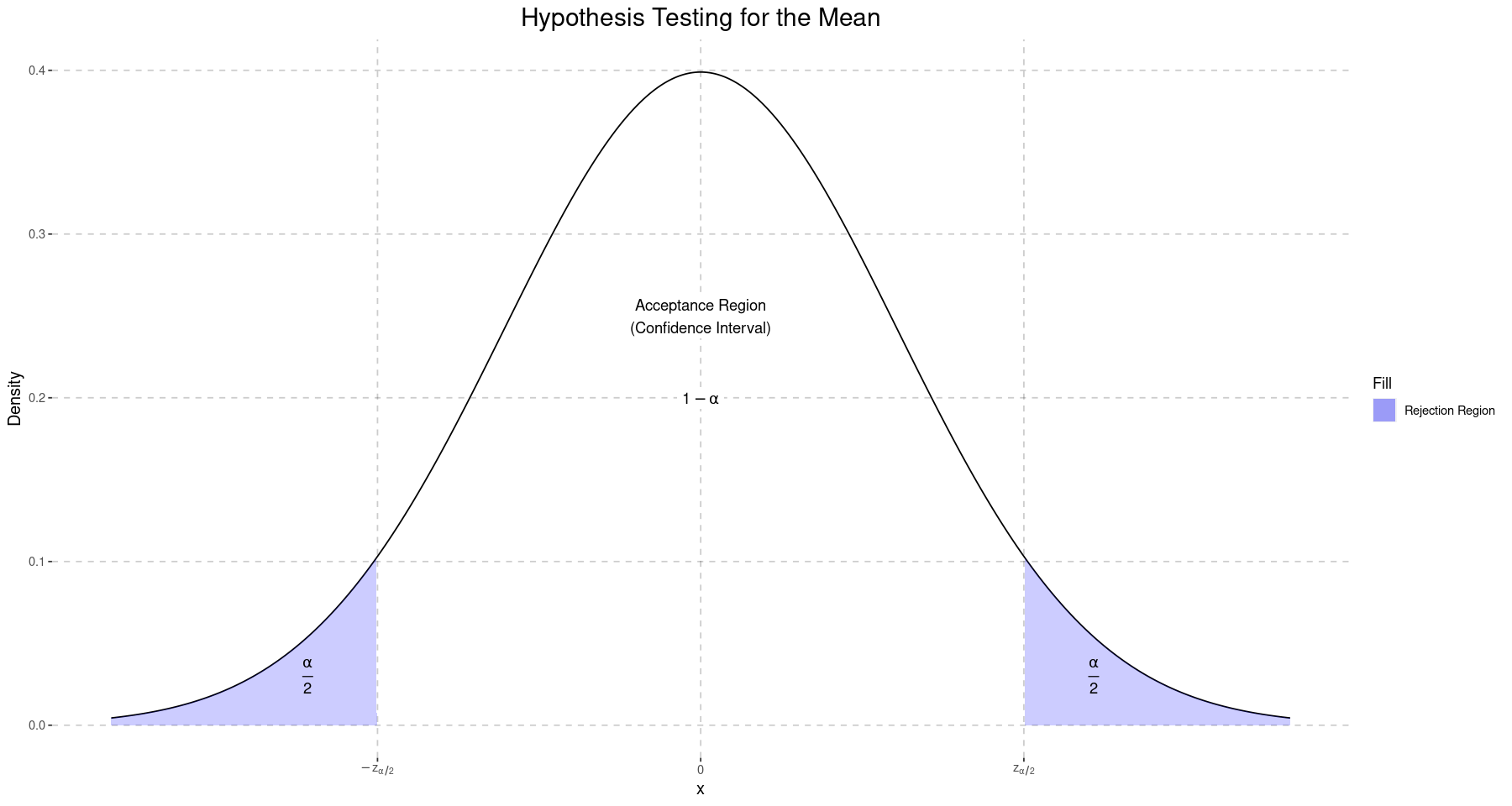
Let’s look at an example to illustrate this point.
Example
A random sample of 100 deaths during the last year in the United States showed an average life span of 71.8 years with a standard deviation of 8.9 years. Does this indicate that the average life span today is greater than 70 years? Use a 0.05 significance level.
(Adapted from Walpole & Myers (1985), ex. 8.3, p. 275)
Our null hypothesis is : , against the one-sided alternative hypothesis : . This is slightly different from the case discussed earlier, since this is a one-sided test rather than a two-sided one, but the same process still applies.
mu <- 70
x_bar <- 71.8
s <- 8.9
n <- 100

z <- (x_bar - mu) / (s / sqrt(n))
z
2.02247191011236
Our value is 2.02, and so now we want to see if that is in the confidence interval. Since this is a 1-sided test, we need at the appropriate level.
alpha <- 0.05
z_alpha <- qnorm(alpha, lower.tail=FALSE)
z_alpha
1.64485362695147
Since our test statistic , we are outside the confidence interval (acceptance regions) and so reject the null hypothesis, concluding that the lifespan is greater than 70 years. We can also be more precise:
p <- pnorm(z, lower.tail = FALSE)
p
0.0215638113390889
Since , we reject . We can also interpret this graphically.
x <- seq(-3, 3, by=0.01)
y <- dnorm(x, mean=0, sd=1)
plot_df <- data.frame(x=x, y=y)

ggplot(plot_df, aes(x, y)) +
    geom_line() +
    annotate('text', x=z+0.2, y=0.02, label=expression(P)) +
    geom_area(data=plot_df[plot_df$x > z,], fill='blue', alpha=0.2) +
    geom_vline(aes(xintercept=0), linetype='dotted') +
    scale_x_continuous(
        breaks=c(0, z_alpha, z),
        labels=c(0, expression(z[alpha]), expression(z))) +
    scale_fill_manual(values="blue") +
    labs(x='x', y='Density', title="Hypothesis Testing for the Mean") +
    personal_theme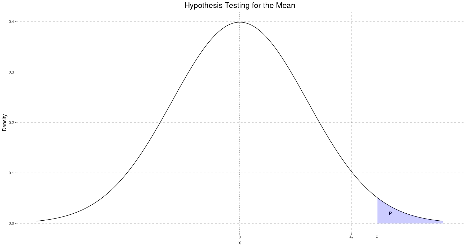
Testing (small samples)
This process was fine because we assumed that we had a large sample size, and specifically one that was large enough for us to credibly substitute for . If we have a small sample size, then the quantity
that is, it has a Student- distribution with degrees of freedom. Otherwise, however, the process remains the same: set our significance level, calculate the value of our test statistic, and see whether it is less than our significance level.
Example
The Edison Electric Institute publishes figures on the annual energy needs of difference appliances, claiming in particular that a certain vacuum cleaner brand expends 46 kilowatt-hours a year. A random sample of 12 homes found an average of 42 kWh with a standard deviation of 11.9 kWh. At a significance level of 0.05, can we conclude that the spend less than 46 kWh annually?
(Adapted from Walpole & Myers (1985) ex. 8.5, p. 278)
Our null hypothesis is : against the alternate hypothesis : . Since the number of homes is small, we use the statistic.
alpha <- 0.05
mu_0 <- 46
n = 12
x_bar <- 42
s <- 11.9

t_alpha <- qt(alpha, n-1, lower.tail=TRUE) # -1.7958...; negative because we are testing the left tail
t <- (x_bar - mu_0) / (s / sqrt(n)) # -1.16...
paste('t_alpha=', t_alpha, ' t=', t)
‘t_alpha= -1.79588481870404 t= -1.16440390424798’
Since our test statistic is greater than our critical value (), we fail to reject the null hypothesis and can therefore not conclude that the annual power usage is less than 46 kWh.
Using values,
pt(t, df=n-1, lower.tail=TRUE)0.134446412758992
Since this value is larger than the desired level of significance , we fail to reject the null hypothesis.
Testing , and Unknown but Equal
Example
Two different kinds of laminated material are being tested by putting them through a machine and then seeing how worn they become. Twelve pieces of material 1 were tested and found to have an average wear of 85 units with a standard deviation of 4, while for material 2 10 pieces were tested and found to have a mean wear of 81 units with a standard deviation of 5. At the 0.05 level, can we conclude that the wear of material 1 exceeds that of material 2 by more than 2 units? Assume the populations to be normal with equal variances.
(Adapted from Walpole & Myers (1985) ex. 8.6, p. 279)
We are testing the null hypothesis : against the alternate hypothesis : . Since we assume that the populations have the same variance, we find an expression for the pooled variance from that of the different samples and use that in our calculation, and so our sample statistic is
where
Since we are testing at the level, we want our test statistic to be greater than .
alpha <- 0.05

n_1 <- 12
x_bar_1 <- 85
s_1 <- 4

n_2 <- 10
x_bar_2 <- 81
s_2 <- 5

d <- 2 # difference we are testing against

df <- n_1 + n_2 - 2 # 20

t_alpha <- qt(alpha, df=df, lower.tail = FALSE) # 1.7247...
s_p <- sqrt(((n_1 - 1)*s_1^2 + (n_2 - 1)*s_2^2) / df) # 4.47...
t <- (( x_bar_1 - x_bar_2 ) - d) / (s_p * sqrt(1 / n_1 + 1 / n_2)) # 1.04
Since our statistic did not exceed at our desired significance level, we fail to reject the null hypothesis and cannot then conclude that the difference is greater than 2.
Using values,
pt(t, df=df, lower.tail=FALSE)0.154659409955889
By the same logic, since this is greater than 0.05 (the desired significance level), we fail to reject the null.
Testing with Paired Observations
Example
In “Influence of physical restraint and restraint-facilitating drugs on blood measurements of white-tailed deer and other selected mammals”, the author examined the effect of succinyl-choline on deer. They were captured (using a dart gun) and the levels of androgen in their blood were checked, and then checked again after 30 minutes, after which point the deer were released. At the 0.05 level of significance, can we conclude that the androgen levels were altered by the drug injection?
| Deer | Time of Injection | 30 minutes after |
|---|---|---|
| 1 | 2.76 | 7.02 |
| 2 | 5.18 | 3.10 |
| 3 | 2.68 | 5.44 |
| 4 | 3.05 | 3.99 |
| 5 | 4.10 | 5.21 |
| 6 | 7.05 | 10.26 |
| 7 | 6.60 | 13.91 |
| 8 | 4.79 | 18.53 |
| 9 | 7.39 | 7.91 |
| 10 | 7.30 | 4.85 |
| 11 | 11.78 | 11.10 |
| 12 | 3.90 | 3.74 |
| 13 | 26.00 | 94.03 |
| 14 | 67.48 | 94.03 |
| 15 | 17.04 | 41.70 |
(Modified from Walpole & Myers (1985), ex. 8.7, p. 280)
Here we want to test not the individual values, but instead their differences. We can use the statistics, since
We are testing the null hypothesis : against the alternate hypothesis . Since this is a two-tailed test (we are testing if the subsequent to the injection the levels rose or fell), we will reject the null if or . Since we are testing at the 0.05 significance level, .
deer_df <- data.frame(
    before=c(
        2.76,
        5.18,
        2.68,
        3.05,
        4.10,
        7.05,
        6.60,
        4.79,
        7.39,
        7.30,
        11.78,
        3.90,
        26.00,
        67.48,
        17.04
    ),
    after=c(
        7.02,
        3.10,
        5.44,
        3.99,
        5.21,
        10.26,
        13.91,
        18.53,
        7.91,
        4.85,
        11.10,
        3.74,
        94.03,
        94.03,
        41.70
    )
)

deer_df$d <- deer_df$after - deer_df$before
deer_df| before | after | d |
|---|---|---|
| <dbl> | <dbl> | <dbl> |
| 2.76 | 7.02 | 4.26 |
| 5.18 | 3.10 | -2.08 |
| 2.68 | 5.44 | 2.76 |
| 3.05 | 3.99 | 0.94 |
| 4.10 | 5.21 | 1.11 |
| 7.05 | 10.26 | 3.21 |
| 6.60 | 13.91 | 7.31 |
| 4.79 | 18.53 | 13.74 |
| 7.39 | 7.91 | 0.52 |
| 7.30 | 4.85 | -2.45 |
| 11.78 | 11.10 | -0.68 |
| 3.90 | 3.74 | -0.16 |
| 26.00 | 94.03 | 68.03 |
| 67.48 | 94.03 | 26.55 |
| 17.04 | 41.70 | 24.66 |
alpha <- 0.05

n <- nrow(deer_df) # 15
df <- n - 1 # 14
d_bar <- mean(deer_df$d) # 9.848
s_d <- sd(deer_df$d) # 18.47

t_alpha_2 <- qt(alpha / 2, df=df, lower.tail = FALSE) # 2.14478... critical value

d <- 0 # null hypothesis difference

t <- (d_bar - d) / (s_d / sqrt(n)) # 2.06
Since our test statistics was not in the rejection region ( or ), we fail to reject the null hypothesis and cannot therefore conclude at the 0.05 significance level that there was a difference in androgen levels before and after the injection.
Alternatively, we could check against the level:
pt(t, df, lower.tail = FALSE)0.0289991646967756
Since this is greater than , we again fail to reject the null.
Conclusion
Although this post was largely going through a series of examples of hypothesis tests which somehow involved either the mean or the difference of means, hopefully the commonalities are starting to become clear. In all cases, we start with our null hypothesis and alternate hypothesis, and then create a confidence interval for the desired quantity (mean or difference of means) at the desired confidence level. We then test to see if our test statistic is within the confidence interval (in which case we fail to reject the null) or outside of it (in which case we reject the null).
Alternatively, this process is exactly equivalent to calculating a value - that is, the probability that we would see data at least as extreme as what we actually witnessed if the null hypothesis were true - and rejecting the null if the data is more extreme than our level of significance or failing to reject it if not.
Bibliography
- Walpole, R. E., & Myers, R. H. (1985). Probability and Statistics for Engineers and Scientists. Macmillan USA.
- Wesson, J. A. (1976). Influence of physical restraint and restraint-facilitating drugs on blood measurements of white-tailed deer and other selected mammals [Virginia Tech]. https://vtechworks.lib.vt.edu/items/bb63de27-3f60-4d17-bff8-2a5a38e1b2b0