Hierarchical Bayesian Models
A look at hierarchical models, a kind of model that allows you to share information between different clusters of data. We'll start with a simple example and then apply it to a real-world situation.
Recently I’ve been learning about multilevel models. These are a kind of model where, by clustering the data in some way, you can ‘share’ information between different pieces of the model. That makes them an excellent way to get the most out of the often limited data that you might have available. Another advantage of these models is that it provides a way to account for additional uncertainty, in much the same way that a mixture model does. Let’s go through and see how to construct such a model (specifically, a varying-intercepts model) and cap it off with a real-world application!
Example - Heights
Let’s start off with a relatively simple example. We’re going to look at the simulated heights of people in different countries. In this situation, there is a natural hierarchical nature to the data: each height belongs to a person and each student belongs to a country. We might naturally expect that the country that a person is part of will have some influence on their score. There are a few ways that we could approach this:
- Ignore the countries We could just ignore the fact that the people are in different countries and group them all together when making our model. This approach is called complete pooling.
- Fit separate models Another approach would be to fit a separate model to each country completely independently. This is the no pooling approach.
At least in this case, both of those seem unsatisfactory. It seems very likely that there is some similarity between the countries - if you learn the mean for one country, that might influence your belief about the next country you visit. So how can we incorporate that information? Essentially, we’re going to fit a model for each country, but each one will share a common prior. This prior will be influenced by the data, and since it is shared between each country that will allow the information from one country to influence the model for the others.
This approach, where we share some information between the different clusters (countries, in this case) is called partial pooling. In the case where there is a hierarchical structure to the data, we call it a hierarchical model.
Let’s try this on some simulated data to see how it works before we apply it to some real data on diploma exam results in Alberta.
Simulation
First let’s set up the situation. For simplicity, we’ll assume that each person’s height is drawn from a normal distribution, and that the mean of that distribution is specific to each country. However, we’ll also assume that the means for the different countries are drawn from a common distribution as well. This will show up in the model as a shared prior.
Let’s use this process to generate some data, and then we’ll use the same model to recover it.
# Set up the environment
library(ggplot2)
library(cmdstanr)
library(posterior)
library(readxl)

options(repr.plot.width = 17, repr.plot.height = 8)set.seed(500)
# country parameters
NUM_COUNTRIES <- 4
country_means <- rnorm(NUM_COUNTRIES, 176, 10)
country_sigma <- rexp(1, 1)
# now generate some people
NUM_PEOPLE <- 20
country_data <- data.frame(
country_index = as.factor(rep(1:NUM_COUNTRIES, each = NUM_PEOPLE)),
height = rnorm(
n = NUM_COUNTRIES * NUM_PEOPLE,
mean = rep(country_means, each = NUM_PEOPLE),
sd = 3
)
)
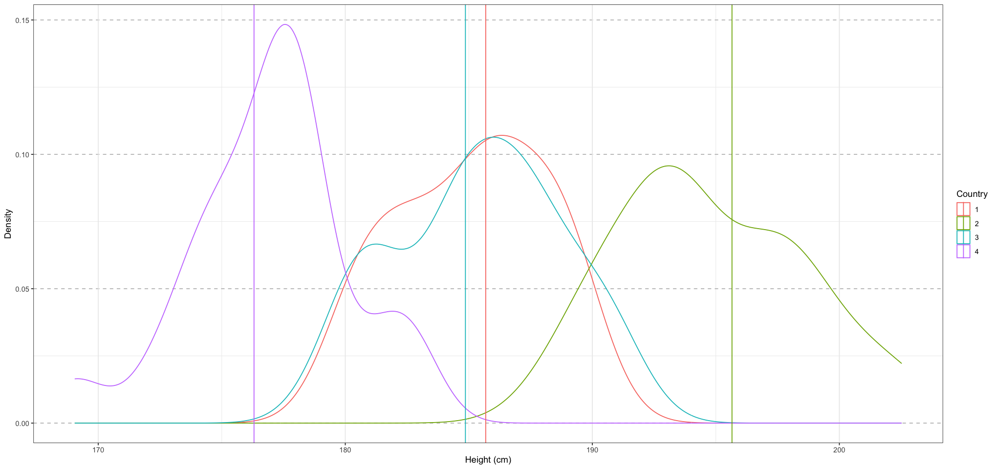
ggplot(country_data, aes(height)) +
geom_density(aes(group = country_index, colour = country_index)) +
geom_vline(data = data.frame(country = as.factor(1:NUM_COUNTRIES), mean = country_means), mapping = aes(xintercept = mean, colour = country)) +
labs(x = "Height (cm)", y = "Density", colour = "Country") +
theme_bw() + # Set background to white
theme(
panel.grid.major.y = element_line(size = 0.5, linetype = 'dashed', colour = "grey")
)
To recover the values, let’s use the following model.
The way that we’re going to share the information between the countries is through the parameter. Because this mean value for the prior for each country must be the same for each of the different countries, it provides a way for that data to flow between them as the model is fit.
Now that we have the data and know the generative process behind it, let’s ensure that we can recover those same values using the model.
stan_model_code <- "
data {
    int<lower = 0> N_COUNTRIES; // number of countries
    int<lower = 0> N; // number of people
    vector[N] heights;
    array[N] int<lower = 0, upper = N_COUNTRIES> country_id; // the country id corresponding to each height
}
parameters {
    vector[N_COUNTRIES] mu_country;
    real<lower = 1e-3> sigma; // sd for the heights
    real<lower = 1e-3> sigma_country; // sd for the country mean values
    real alpha_bar;
}
model {
    heights ~ normal(mu_country[country_id], sigma);
    mu_country ~ normal(alpha_bar, 10);
    alpha_bar ~ normal(176, 1);
    sigma_country ~ exponential(1);
    sigma ~ exponential(1);
}
"
stan_model_file <- write_stan_file(stan_model_code)
stan_model <- cmdstan_model(stan_model_file)

stan_model_data <- list(
    N_COUNTRIES = NUM_COUNTRIES,
    N = nrow(country_data),
    heights = country_data$height,
    country_id = as.integer(country_data$country_index)
)
fit <- stan_model$sample(
    data = stan_model_data,
    chains = 4
)
Running MCMC with 4 sequential chains...
All 4 chains finished successfully.
Mean chain execution time: 0.0 seconds.
Total execution time: 0.5 seconds.fit$summary()| variable | mean | median | sd | mad | q5 | q95 | rhat | ess_bulk | ess_tail |
|---|---|---|---|---|---|---|---|---|---|
| <chr> | <dbl> | <dbl> | <dbl> | <dbl> | <dbl> | <dbl> | <dbl> | <dbl> | <dbl> |
| lp__ | -144.334351 | -143.9545000 | 1.9631562 | 1.7183334 | -148.04970000 | -141.819900 | 1.000846 | 1640.376 | 2355.089 |
| mu_country[1] | 185.073222 | 185.0600000 | 0.7513226 | 0.7405587 | 183.82495000 | 186.320100 | 1.000304 | 6575.682 | 3154.603 |
| mu_country[2] | 194.750996 | 194.7570000 | 0.7414349 | 0.7220262 | 193.50895000 | 195.958100 | 1.001592 | 7044.055 | 2985.646 |
| mu_country[3] | 185.335148 | 185.3370000 | 0.7385066 | 0.6983046 | 184.07985000 | 186.547750 | 1.001719 | 7405.325 | 2834.630 |
| mu_country[4] | 176.916428 | 176.9180000 | 0.7482134 | 0.7650216 | 175.69300000 | 178.154050 | 1.001806 | 6358.099 | 2966.653 |
| sigma | 3.342929 | 3.3194700 | 0.2687868 | 0.2637768 | 2.93077650 | 3.815515 | 1.001739 | 6754.819 | 3248.544 |
| sigma_country | 1.000606 | 0.6943115 | 0.9873734 | 0.7047710 | 0.04307331 | 2.940308 | 1.000265 | 3774.295 | 1877.089 |
| alpha_bar | 176.364408 | 176.3655000 | 0.9784172 | 0.9748095 | 174.74800000 | 177.984050 | 1.000514 | 7930.243 | 2686.251 |
From the summary table, we can see that our posterior values are close to the true values. Let’s see the same thing graphically.
height_draws <- as_draws_matrix(fit)
head(height_draws)| lp__ | mu_country[1] | mu_country[2] | mu_country[3] | mu_country[4] | sigma | sigma_country | alpha_bar | |
|---|---|---|---|---|---|---|---|---|
| 1 | -144.016 | 185.422 | 194.549 | 185.765 | 176.804 | 3.57034 | 0.0527758 | 175.646 |
| 2 | -143.700 | 184.574 | 194.249 | 184.553 | 176.397 | 3.26862 | 3.6745100 | 177.132 |
| 3 | -145.799 | 183.510 | 195.764 | 184.747 | 176.220 | 3.36722 | 0.3739620 | 175.124 |
| 4 | -144.623 | 185.169 | 193.716 | 184.875 | 176.145 | 3.54078 | 1.0502200 | 178.216 |
| 5 | -143.933 | 184.849 | 195.680 | 185.868 | 177.684 | 3.21139 | 0.9323830 | 174.692 |
| 6 | -144.299 | 185.165 | 193.932 | 184.807 | 176.049 | 3.46684 | 1.2301000 | 178.207 |
country_mean_results <- height_draws[, grep('mu_country', colnames(height_draws))]
results_df <- data.frame(
    country_id = 1:NUM_COUNTRIES,
    mean = apply(country_mean_results, 2, mean),
    lower = apply(country_mean_results, 2, function(row) quantile(row, 0.025)),
    upper = apply(country_mean_results, 2, function(row) quantile(row, 0.975)),
    type = "Posterior"
)

posterior_alpha_bar <- mean(height_draws[, 'alpha_bar'])

ggplot(results_df, aes(country_id, mean)) +
    geom_point(aes(colour = type)) +
    geom_errorbar(aes(ymin = lower, ymax = upper)) +
    geom_point(data = data.frame(country_id = 1:NUM_COUNTRIES, mean = country_means, type = "Actual"), mapping = aes(colour = type)) +
    geom_hline(mapping = aes(yintercept = posterior_alpha_bar), linetype = 'dashed') +
    labs(x = "Country", y = "Height (cm)", colour = "Type") +
    theme_bw() +  # Set background to white
    theme(
        panel.grid.major.y = element_line(size = 0.5, linetype = 'dashed', colour = "grey"),
    )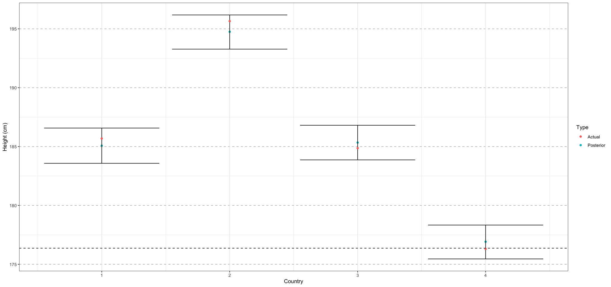
One thing to note is that we have a larger error than we would expect if we fit each country individually. The reason for that is that a hierarchical model like this tends to ‘shrink’ estimates towards the mean. You can see this here by the fact that the values of the posterior tend to be closer to the mean than the actual values. While it may seem crazy to deliberately choose a model that will tend to do worse on the data, in fact this is just part of the overfitting / underfitting tradeoff - by biasing estimates to the mean, we will do worse on our training set but better on outside data.
So now that we’ve seen a relatively simple example, let’s try to build our way towards our eventual goal of applying this idea to school test scores.
Example - School Test Scores
Imagine that you have a number of different schools in a school division, and you’re interested in how the students in those schools are doing on a test. We believe that each school has an effect on the students, and we also believe that the school division has an effect on the school. Here we have two nested pools - each student belongs to a school, and each school belongs to a district.
Simulation
Imagine that you have nine schools taking part in some sort of standardized exam. Each school has some number of students that are taking the exam, and they each get a grade. The grade they get is a combination of luck, their own properties, and some influence of the school. The influence of the school is itself dependent on the school district. Let’s try to generate some data, then create a model to recover the original values. By doing so, we’re ensuring that our model is fit for purpose.
Since this model is a bit more complex, let’s take it one step at a time.
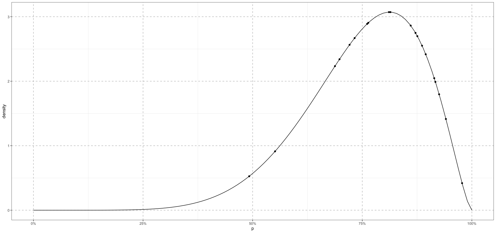
First, let’s start with a single school. The distribution for the school’s students will be drawn from a beta distribution. The beta is the perfect distribution for this since it’s a distribution of probabilities, which is what we’re looking for. The beta distribution has two parameters, and . The mean is , and the variance is . If we’re thinking of the beta distribution as being related to a Binomial random process (i.e. a set of coin flips), then we can think of as the number of successes and as the number of failures. This is not quite correct, but it’s pretty close.
So let’s say that we want the school average to be about 75%. There are a few different values of and that we could choose; we just need the mean . For instance, and would work. So would any multiple of the those: 6 and 2, 4 and , &c.
alpha_base <- 3
beta_base <- 1

multiples <- seq.int(from = 1, to = 4)
plot_df <- data.frame(p = numeric(), density = numeric(), type = character())

probs <- seq(from = 0, to = 1, length.out = 100)
for (multiple in multiples) {
    alpha <- alpha_base * multiple
    beta <- beta_base * multiple
    data <- data.frame(p = probs, density = dbeta(probs, alpha, beta), type = paste("alpha = ", alpha, " beta = ", beta))
    plot_df <- rbind(plot_df, data)
}

ggplot(plot_df, aes(p, density, group = type, colour = type)) +
    geom_line() +
    labs(x = "p", y = "Density", colour = "Parameter Values") +
    scale_x_continuous(labels = scales::percent_format(accuracy = 1)) +
    theme_bw() +  # Set background to white
    theme(
        panel.grid.major = element_line(size = 0.5, linetype = 'dashed', colour = "grey"),
    )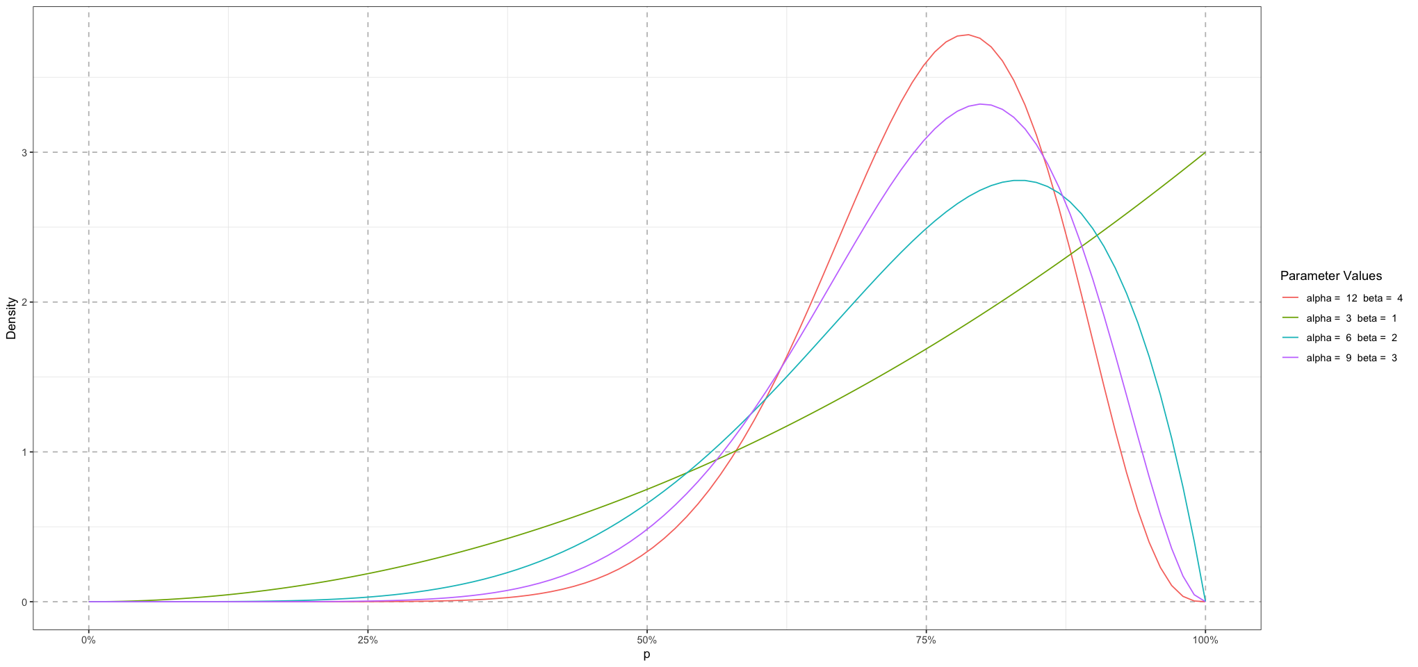
Note that although the mean for each of these is at , that’s not the same as having the peak value be there.
If we’re thinking forward to making our model, it’s not clear to me exactly what we should be thinking of the parameters and as representing. Intuitively, I’d prefer to think in terms of the mean and variance (or even more generally, the centre and the spread) of the expected data. Luckily, it turns out that there is a reparameterization of the beta in terms of these:
Solving for and ,
Let’s recreate the above using this parameterization to convince ourselves that it works. Since we’re fixing our mean, the spread parameter is the only one that needs to change.
mu <- 0.75
spread <- 4 # 'sample size'

plot_df <- data.frame(p = numeric(), density = numeric(), type = character())

probs <- seq(from = 0, to = 1, length.out = 100)
for (sample_size in seq.int(from = 4, to = 16, by = 4)) {
    alpha <- mu * sample_size
    beta <- (1 - mu) * sample_size
    data <- data.frame(p = probs, density = dbeta(probs, alpha, beta), type = paste("mu = ", mu, " nu = ", sample_size))
    plot_df <- rbind(plot_df, data)
}

ggplot(plot_df, aes(p, density, group = type, colour = type)) +
    geom_line() +
    labs(x = "p", y = "Density", colour = "Parameter Values") +
    scale_x_continuous(labels = scales::percent_format(accuracy = 1)) +
    theme_bw() +  # Set background to white
    theme(
        panel.grid.major = element_line(size = 0.5, linetype = 'dashed', colour = "grey"),
    )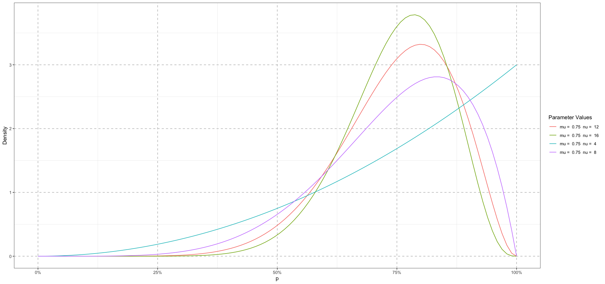
Great! So now we have our parameterization. Let’s make sure that we can model at least this part of the problem. Let’s say that we have a school where the average test score is 75%, and let’s simulate a class of 20 students.
NUM_STUDENTS <- 20
school_mu <- 0.75
school_nu <- 10 # this is *not* the same as the number of students!

alpha <- school_mu * school_nu
beta <- (1 - school_mu) * school_nu

actual_student_scores <- rbeta(NUM_STUDENTS, alpha, beta)

p <- seq(from = 0, to = 1, length.out = 100)
line_data <- data.frame(p = p, density = dbeta(p, alpha, beta))
student_data <- data.frame(p = actual_student_scores, density = dbeta(actual_student_scores, alpha, beta))
ggplot() +
    geom_line(data = line_data, mapping = aes(p, density)) +
    geom_point(data = student_data, mapping = aes(p, density)) +
    scale_x_continuous(labels = scales::percent_format(accuracy = 1)) +
    theme_bw() +
    theme(
        panel.grid.major = element_line(size = 0.5, linetype = 'dashed', colour = "grey"),
    )
So here we can see the theoretical distribution of the students’ scores along with the actual scores. Now let’s use a model to recover those values!
How did we arrive at those priors? We ran some simulations of the model with different parameters to find ones that were reasonable. In a real model we would do this before looking at the data, but in this case that’s not really possible. We’ll just pretend that we don’t know what the data should look like. Also, when checking a model like this, it’s not unreasonable to start with a model that reflects the true underlying process - the idea here is that we are ground-truthing it. If the model can’t get back the correct values even when we know the model is correct and the values are close, then it really isn’t fit for purpose.
NUM_SIM_STUDENTS <- 100
nu <- rnorm(NUM_SIM_STUDENTS, 10, 1)
mu <- rbeta(NUM_SIM_STUDENTS, 12, 4)
alpha <- mu * nu
beta <- (1 - mu) * nu
s <- rbeta(NUM_SIM_STUDENTS, alpha, beta)

plot_df <- data.frame(s = s)
ggplot(plot_df, aes(s)) +
    geom_density() +
    labs(x = "Score", y = "Density") +
    coord_cartesian(xlim = c(0, 1)) +
    scale_x_continuous(labels = scales::percent_format(accuracy = 1)) +
    theme_bw() +
    theme(
        panel.grid.major = element_line(size = 0.5, linetype = 'dashed', colour = "grey"),
    )
ggplot(data.frame(nu = nu), aes(nu)) +
    geom_density() +
    scale_x_continuous(labels = scales::percent_format(accuracy = 1)) +
    labs(x = "Score", y = "Density") +
    theme_bw() +
    theme(
        panel.grid.major = element_line(size = 0.5, linetype = 'dashed', colour = "grey"),
    )
Before we do anything else, let’s do a prior predictive check. The idea here is to see what kind of values our model is producing before we feed it any data. In large part this should help to constrain our priors - are the data that we’re seeing come out of the model in line with our expectations? Are they plausible? If not, we’ll have to go back and revise our priors. We can actually use Stan to help us with this.
student_score_model_pp_code <- "
data {
    int<lower = 0> N; // number of students
}
parameters {
    real<lower = 0, upper = 1> mu;
    real<lower = 0> nu;
}
 transformed parameters {
    real<lower = 0> a = mu * nu;
    real<lower = 0> b = (1 - mu) * nu;
}
model {
    mu ~ beta(12, 4);
    nu ~ normal(10, 1);
}
generated quantities {
    vector[N] s_sim;
    for (n in 1:N) {
        s_sim[n] = beta_rng(a, b);
    }
}
"

student_score_model_pp_file <- write_stan_file(student_score_model_pp_code)
student_score_pp_model <- cmdstan_model(student_score_model_pp_file)

student_score_model_pp_data <- list(
    N = 100
)

student_score_pp_fit <- student_score_pp_model$sample(
    data = student_score_model_pp_data,
    chains = 4
)
student_score_pp_fit$summary()
Running MCMC with 4 sequential chains...
All 4 chains finished successfully.
Mean chain execution time: 0.0 seconds.
Total execution time: 0.5 seconds.| variable | mean | median | sd | mad | q5 | q95 | rhat | ess_bulk | ess_tail |
|---|---|---|---|---|---|---|---|---|---|
| <chr> | <dbl> | <dbl> | <dbl> | <dbl> | <dbl> | <dbl> | <dbl> | <dbl> | <dbl> |
| lp__ | -7.7472137 | -7.3961950 | 1.1037489 | 0.7291056 | -10.0643700 | -6.7499540 | 1.0005178 | 1726.762 | 1776.441 |
| mu | 0.7536242 | 0.7642695 | 0.1042146 | 0.1057909 | 0.5686431 | 0.9068932 | 1.0015275 | 3183.736 | 1685.494 |
| nu | 9.9871312 | 10.0048000 | 1.0097168 | 0.9897838 | 8.2924295 | 11.6080150 | 1.0008779 | 3470.894 | 2249.882 |
| a | 7.5237364 | 7.5277800 | 1.2812031 | 1.2879643 | 5.3965645 | 9.6125255 | 1.0006855 | 3423.556 | 2280.696 |
| b | 2.4633951 | 2.3360800 | 1.0812236 | 1.0767531 | 0.8796699 | 4.3757240 | 1.0014289 | 3148.109 | 1744.702 |
| s_sim[1] | 0.7519102 | 0.7771395 | 0.1645582 | 0.1691661 | 0.4368936 | 0.9719049 | 0.9997345 | 3638.240 | 3666.031 |
| s_sim[2] | 0.7511981 | 0.7766295 | 0.1655453 | 0.1734783 | 0.4370754 | 0.9752769 | 1.0019282 | 3536.600 | 2732.750 |
| s_sim[3] | 0.7534096 | 0.7796105 | 0.1623245 | 0.1685798 | 0.4469912 | 0.9749123 | 1.0000188 | 3211.546 | 2890.503 |
| s_sim[4] | 0.7516449 | 0.7772990 | 0.1643784 | 0.1697799 | 0.4385267 | 0.9744425 | 0.9998382 | 3465.035 | 3140.728 |
| s_sim[5] | 0.7500511 | 0.7759265 | 0.1690192 | 0.1730068 | 0.4296476 | 0.9745945 | 1.0011223 | 3213.409 | 2759.927 |
| s_sim[6] | 0.7546354 | 0.7789480 | 0.1622561 | 0.1683270 | 0.4521205 | 0.9721189 | 1.0016519 | 3591.587 | 2984.244 |
| s_sim[7] | 0.7550554 | 0.7788565 | 0.1603555 | 0.1662313 | 0.4607637 | 0.9725681 | 1.0003974 | 3557.438 | 2779.617 |
| s_sim[8] | 0.7549163 | 0.7815435 | 0.1658129 | 0.1695472 | 0.4389618 | 0.9750677 | 0.9996789 | 3018.343 | 2864.190 |
| s_sim[9] | 0.7557622 | 0.7824510 | 0.1628229 | 0.1724256 | 0.4547386 | 0.9739696 | 1.0000825 | 3615.700 | 3202.578 |
| s_sim[10] | 0.7580823 | 0.7858460 | 0.1645778 | 0.1722047 | 0.4479410 | 0.9737689 | 0.9997881 | 3390.171 | 3311.547 |
| s_sim[11] | 0.7526162 | 0.7805120 | 0.1665224 | 0.1725220 | 0.4385346 | 0.9756622 | 1.0006392 | 3648.114 | 3135.257 |
| s_sim[12] | 0.7547576 | 0.7769915 | 0.1628121 | 0.1683196 | 0.4495085 | 0.9720077 | 0.9997057 | 3701.263 | 3590.140 |
| s_sim[13] | 0.7549515 | 0.7827305 | 0.1646374 | 0.1691936 | 0.4403020 | 0.9741046 | 1.0009201 | 3463.333 | 3247.366 |
| s_sim[14] | 0.7562782 | 0.7825465 | 0.1624611 | 0.1725020 | 0.4543448 | 0.9743693 | 1.0007592 | 3531.548 | 3317.929 |
| s_sim[15] | 0.7555521 | 0.7797795 | 0.1632866 | 0.1702054 | 0.4528257 | 0.9755237 | 0.9996543 | 3702.652 | 2749.965 |
| s_sim[16] | 0.7554666 | 0.7803640 | 0.1629003 | 0.1675064 | 0.4497360 | 0.9738368 | 0.9997797 | 3369.579 | 3193.877 |
| s_sim[17] | 0.7496401 | 0.7786345 | 0.1679984 | 0.1743945 | 0.4295800 | 0.9750243 | 1.0006391 | 3546.795 | 3577.849 |
| s_sim[18] | 0.7557703 | 0.7809600 | 0.1658010 | 0.1700186 | 0.4469792 | 0.9739523 | 1.0006038 | 3835.557 | 3256.432 |
| s_sim[19] | 0.7559281 | 0.7823020 | 0.1618966 | 0.1639392 | 0.4468340 | 0.9732376 | 0.9996622 | 3645.435 | 2824.582 |
| s_sim[20] | 0.7528602 | 0.7790840 | 0.1680849 | 0.1709890 | 0.4281760 | 0.9750786 | 1.0001791 | 3651.577 | 3719.415 |
| s_sim[21] | 0.7523741 | 0.7761915 | 0.1644295 | 0.1704575 | 0.4476327 | 0.9764495 | 0.9997132 | 3746.216 | 3333.132 |
| s_sim[22] | 0.7561313 | 0.7855385 | 0.1638816 | 0.1694990 | 0.4448916 | 0.9734162 | 1.0009543 | 3417.160 | 2777.871 |
| s_sim[23] | 0.7499353 | 0.7768145 | 0.1655774 | 0.1709453 | 0.4405739 | 0.9753409 | 1.0001462 | 3678.281 | 2928.156 |
| s_sim[24] | 0.7507685 | 0.7770365 | 0.1643030 | 0.1680290 | 0.4446655 | 0.9708647 | 0.9996292 | 2999.935 | 3179.589 |
| s_sim[25] | 0.7539305 | 0.7809975 | 0.1634029 | 0.1679719 | 0.4425114 | 0.9729435 | 1.0006023 | 3634.668 | 3420.166 |
| ⋮ | ⋮ | ⋮ | ⋮ | ⋮ | ⋮ | ⋮ | ⋮ | ⋮ | ⋮ |
| s_sim[71] | 0.7523116 | 0.7806950 | 0.1657678 | 0.1687421 | 0.4386995 | 0.9737648 | 1.0013223 | 3680.581 | 2971.260 |
| s_sim[72] | 0.7583762 | 0.7842995 | 0.1617939 | 0.1736006 | 0.4545544 | 0.9710739 | 0.9996976 | 3301.585 | 2840.791 |
| s_sim[73] | 0.7556720 | 0.7820165 | 0.1627936 | 0.1684300 | 0.4478169 | 0.9726397 | 1.0012680 | 3499.080 | 3208.706 |
| s_sim[74] | 0.7547181 | 0.7809220 | 0.1610201 | 0.1644411 | 0.4516467 | 0.9715066 | 1.0000198 | 3399.117 | 3014.405 |
| s_sim[75] | 0.7533381 | 0.7742685 | 0.1628741 | 0.1689408 | 0.4496273 | 0.9764632 | 1.0006530 | 3359.687 | 3042.876 |
| s_sim[76] | 0.7532482 | 0.7778980 | 0.1649907 | 0.1723345 | 0.4448392 | 0.9764751 | 1.0001158 | 3729.772 | 3561.618 |
| s_sim[77] | 0.7540697 | 0.7776255 | 0.1620004 | 0.1687421 | 0.4493149 | 0.9748428 | 0.9999781 | 3709.743 | 2924.111 |
| s_sim[78] | 0.7552318 | 0.7787180 | 0.1617609 | 0.1699089 | 0.4518985 | 0.9716803 | 1.0002355 | 3542.855 | 3354.554 |
| s_sim[79] | 0.7513719 | 0.7772095 | 0.1658203 | 0.1766436 | 0.4388728 | 0.9748116 | 1.0006742 | 3688.171 | 3517.024 |
| s_sim[80] | 0.7554185 | 0.7786930 | 0.1624798 | 0.1663314 | 0.4521462 | 0.9719680 | 1.0010131 | 3649.007 | 3431.718 |
| s_sim[81] | 0.7529500 | 0.7810250 | 0.1663739 | 0.1738519 | 0.4480554 | 0.9728977 | 0.9997702 | 3675.678 | 3117.200 |
| s_sim[82] | 0.7584932 | 0.7843625 | 0.1628715 | 0.1717866 | 0.4469598 | 0.9736029 | 1.0007292 | 3708.661 | 2922.429 |
| s_sim[83] | 0.7551523 | 0.7812750 | 0.1621680 | 0.1705917 | 0.4538208 | 0.9739764 | 0.9998353 | 3542.688 | 3206.694 |
| s_sim[84] | 0.7517418 | 0.7747835 | 0.1657026 | 0.1712974 | 0.4443958 | 0.9745813 | 1.0003951 | 3590.600 | 3007.862 |
| s_sim[85] | 0.7546482 | 0.7788100 | 0.1613026 | 0.1697799 | 0.4558926 | 0.9730513 | 1.0003160 | 3801.188 | 3413.002 |
| s_sim[86] | 0.7567569 | 0.7850845 | 0.1637229 | 0.1612750 | 0.4398513 | 0.9756185 | 1.0008255 | 3110.995 | 3298.655 |
| s_sim[87] | 0.7539145 | 0.7805230 | 0.1656245 | 0.1711195 | 0.4407317 | 0.9758564 | 0.9999048 | 3385.537 | 3236.119 |
| s_sim[88] | 0.7532113 | 0.7794330 | 0.1635724 | 0.1741670 | 0.4490222 | 0.9743499 | 1.0008099 | 3492.836 | 3293.382 |
| s_sim[89] | 0.7517793 | 0.7806965 | 0.1663839 | 0.1742381 | 0.4344092 | 0.9739365 | 1.0005292 | 3617.638 | 3039.248 |
| s_sim[90] | 0.7536933 | 0.7797350 | 0.1630973 | 0.1666465 | 0.4467467 | 0.9694501 | 0.9997169 | 3493.019 | 3535.025 |
| s_sim[91] | 0.7573752 | 0.7821005 | 0.1613137 | 0.1701543 | 0.4571854 | 0.9733186 | 1.0001893 | 3728.733 | 2855.958 |
| s_sim[92] | 0.7499069 | 0.7755345 | 0.1668960 | 0.1723574 | 0.4416318 | 0.9717048 | 1.0002116 | 3454.466 | 2728.611 |
| s_sim[93] | 0.7544595 | 0.7786440 | 0.1623672 | 0.1724004 | 0.4516196 | 0.9726107 | 1.0008192 | 3533.927 | 3457.289 |
| s_sim[94] | 0.7578421 | 0.7856785 | 0.1638296 | 0.1698348 | 0.4472335 | 0.9747376 | 0.9999161 | 3605.345 | 3350.634 |
| s_sim[95] | 0.7530364 | 0.7766930 | 0.1627019 | 0.1702551 | 0.4503490 | 0.9751747 | 1.0001220 | 3690.476 | 2992.951 |
| s_sim[96] | 0.7544495 | 0.7785435 | 0.1628462 | 0.1691906 | 0.4541267 | 0.9745491 | 0.9999704 | 3711.595 | 3040.620 |
| s_sim[97] | 0.7531373 | 0.7830350 | 0.1628663 | 0.1649704 | 0.4441329 | 0.9745094 | 1.0005597 | 3653.499 | 3222.520 |
| s_sim[98] | 0.7550406 | 0.7807990 | 0.1623796 | 0.1687466 | 0.4426782 | 0.9725074 | 0.9997867 | 3655.128 | 3620.627 |
| s_sim[99] | 0.7545676 | 0.7812840 | 0.1648859 | 0.1710935 | 0.4401541 | 0.9733861 | 0.9995537 | 3310.877 | 3100.817 |
| s_sim[100] | 0.7513484 | 0.7802295 | 0.1663923 | 0.1774435 | 0.4426189 | 0.9735879 | 1.0006365 | 3509.837 | 3482.959 |
From the above summary the values of the parameters mu and nu look correct, as do the values for the simulated student scores. The rhat for each parameter also looks good (close to 1) and the effective sample size (ess_bulk) is also good. There was a minor problem in the fitting where a nan value was generated, but that’s a rare thing and only happens intermittently. Overall, this looks good! Now let’s get the data.
draws <- as_draws_matrix(student_score_pp_fit)
head(draws)| lp__ | mu | nu | a | b | s_sim[1] | s_sim[2] | s_sim[3] | s_sim[4] | s_sim[5] | ⋯ | s_sim[91] | s_sim[92] | s_sim[93] | s_sim[94] | s_sim[95] | s_sim[96] | s_sim[97] | s_sim[98] | s_sim[99] | s_sim[100] | |
|---|---|---|---|---|---|---|---|---|---|---|---|---|---|---|---|---|---|---|---|---|---|
| 1 | -6.95483 | 0.667633 | 9.97229 | 6.65783 | 3.314450 | 0.456435 | 0.664123 | 0.711574 | 0.447643 | 0.734297 | ⋯ | 0.498274 | 0.754939 | 0.726993 | 0.456323 | 0.703468 | 0.969384 | 0.719329 | 0.285399 | 0.578132 | 0.768713 |
| 2 | -8.32990 | 0.657733 | 8.48227 | 5.57907 | 2.903200 | 0.768042 | 0.804358 | 0.498766 | 0.565657 | 0.611261 | ⋯ | 0.665832 | 0.934308 | 0.768160 | 0.528255 | 0.680999 | 0.446552 | 0.549291 | 0.703405 | 0.675308 | 0.620042 |
| 3 | -10.93100 | 0.944694 | 8.70912 | 8.22745 | 0.481670 | 0.999742 | 0.956379 | 0.906580 | 0.895511 | 0.937207 | ⋯ | 0.991936 | 0.811721 | 0.989481 | 0.901462 | 0.982731 | 0.996148 | 0.797290 | 0.964812 | 0.756131 | 0.917414 |
| 4 | -7.77407 | 0.883106 | 10.01070 | 8.84047 | 1.170190 | 0.827503 | 0.868712 | 0.780807 | 0.922841 | 0.902845 | ⋯ | 0.725912 | 0.814534 | 0.861869 | 0.816770 | 0.909844 | 0.965625 | 0.880752 | 0.953130 | 0.911444 | 0.711088 |
| 5 | -8.18839 | 0.899799 | 9.86949 | 8.88056 | 0.988932 | 0.982008 | 0.934849 | 0.971897 | 0.987508 | 0.929194 | ⋯ | 0.996558 | 0.889514 | 0.993364 | 0.945195 | 0.745194 | 0.865354 | 0.919428 | 0.896571 | 0.738742 | 0.974191 |
| 6 | -7.55440 | 0.646480 | 11.06220 | 7.15148 | 3.910700 | 0.676698 | 0.280590 | 0.649463 | 0.611321 | 0.680222 | ⋯ | 0.632214 | 0.426887 | 0.810964 | 0.408792 | 0.752207 | 0.704922 | 0.556105 | 0.785266 | 0.632428 | 0.470659 |
Now that we have the draws, let’s plot a few different classes of 100 students (s_sim) to see what kind of variation the model is producing.
set.seed(2024)
s_sim_draws <- draws[, grep('s_sim', colnames(draws))]
s_sim_means <- mean(apply(s_sim_draws, 2, mean))

p <- ggplot() +
    coord_cartesian(xlim = c(0, 1)) +
    geom_vline(data = data.frame(xintercept = s_sim_means), mapping = aes(xintercept=xintercept)) +
    labs(x = "Score", y = "Density") +
    scale_y_continuous(labels = scales::percent_format(accuracy = 1)) +
    theme_bw() +  # Set background to white
    theme(
        panel.grid.major = element_line(size = 0.5, linetype = 'dashed', colour = "grey"),
    )

for (row in sample(1:4000, size = 100)) {
    data <- data.frame(s = as.vector(s_sim_draws[row, ]))
    p <- p + geom_density(data = data, mapping = aes(s), colour = alpha('black', 0.1))
}

print(p)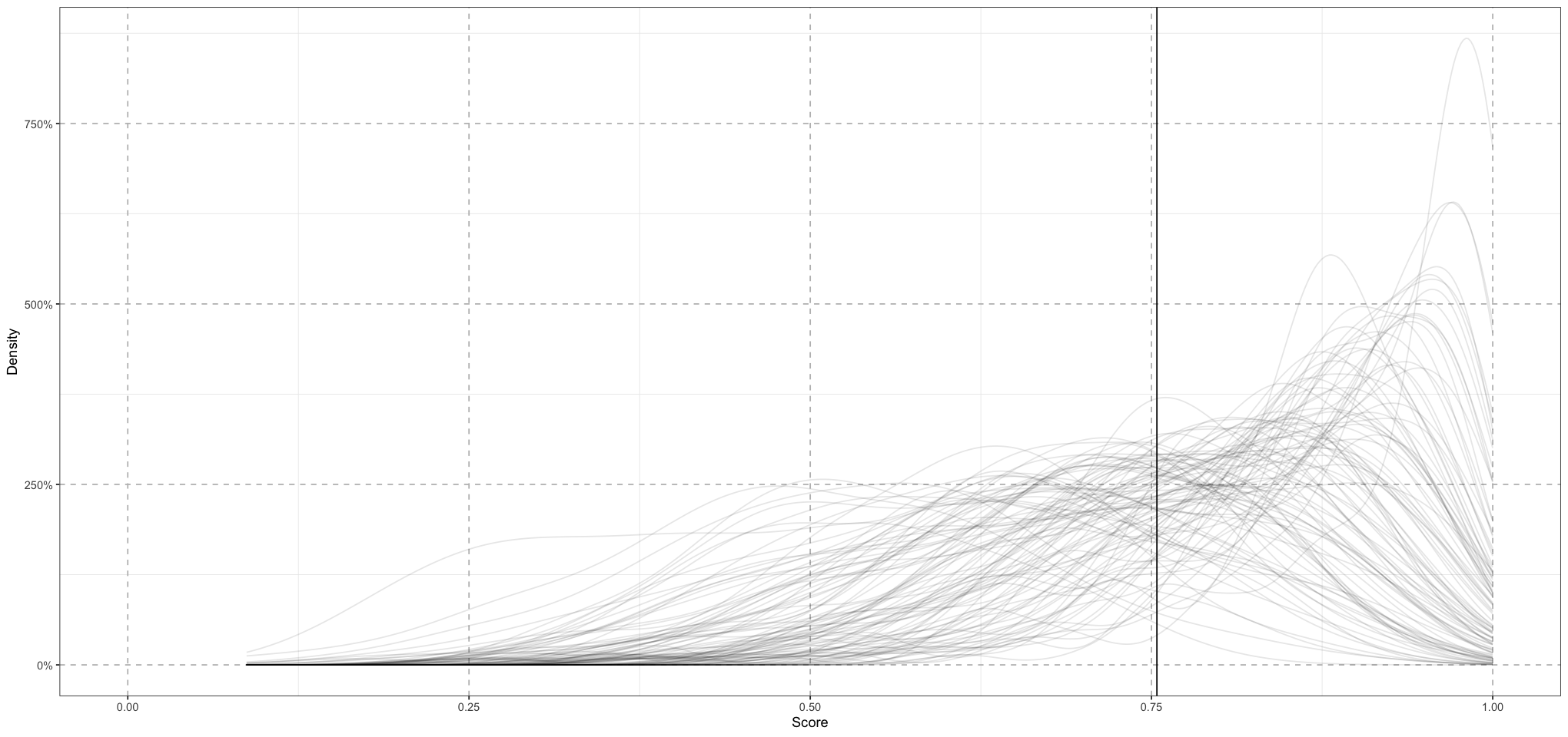
What we see here are the results of 100 randomly chosen simulated classes. This seems roughly reasonable to me - the mean is firmly centred around 75% and there’s considerable variation. Looking at this, there is maybe a bit too much variation - I would expect almost all of the weight to be in the range 50% - 100%, and there are a few classes with a significant amount of weight below 50%. On the other hand, it’s probably not the worst thing in the world for this to have too much variation - the data should be able to fix that.
Now let’s actually train the model on some data and see what happens. We’ll have to slightly modify the model we used for our prior predictive check to incorporate the data, but otherwise it will look very similar.
student_score_model_code <- "
data {
    int<lower = 0> N; // number of students
    vector[N] s; // student scores
}
parameters {
    real<lower = 0, upper = 1> mu;
    real<lower = 0> nu;
}
 transformed parameters {
    real<lower = 0> a = mu * nu;
    real<lower = 0> b = (1 - mu) * nu;
}
model {
    s ~ beta(a, b);
    mu ~ beta(12, 4);
    nu ~ normal(10, 1);
}
"

student_score_model_file <- write_stan_file(student_score_model_code)
student_score_model <- cmdstan_model(student_score_model_file)

student_score_model_data <- list(
    N = NUM_STUDENTS,
    s = actual_student_scores
)
student_score_fit <- student_score_model$sample(
    data = student_score_model_data,
    chains = 4
)
student_score_fit$summary()
Running MCMC with 4 sequential chains...
All 4 chains finished successfully.
Mean chain execution time: 0.0 seconds.
Total execution time: 0.6 seconds.| variable | mean | median | sd | mad | q5 | q95 | rhat | ess_bulk | ess_tail |
|---|---|---|---|---|---|---|---|---|---|
| <chr> | <dbl> | <dbl> | <dbl> | <dbl> | <dbl> | <dbl> | <dbl> | <dbl> | <dbl> |
| lp__ | 7.9908730 | 8.3131950 | 0.9971564 | 0.70121791 | 5.9504810 | 8.9398085 | 1.001998 | 1874.212 | 2717.678 |
| mu | 0.8019337 | 0.8031015 | 0.0247588 | 0.02413969 | 0.7597064 | 0.8411199 | 1.000958 | 2543.792 | 2389.431 |
| nu | 9.9267693 | 9.9146750 | 0.9365335 | 0.93079852 | 8.4171405 | 11.4982400 | 1.000450 | 3232.958 | 2479.932 |
| a | 7.9625121 | 7.9612550 | 0.8081238 | 0.81650489 | 6.6524980 | 9.3088245 | 0.999826 | 3037.912 | 2657.738 |
| b | 1.9642571 | 1.9528450 | 0.2943620 | 0.29113816 | 1.4906390 | 2.4721195 | 1.001831 | 3197.077 | 2450.331 |
draws <- as_draws_matrix(student_score_fit)

# mu
ggplot(data.frame(mu = draws[, 'mu'])) +
    geom_density(aes( mu )) +
    geom_vline(aes(xintercept = 0.75)) +
    coord_cartesian(xlim = c(0, 1)) +
    labs(x = "mu", y = "Density") +
    scale_x_continuous(labels = scales::percent_format(accuracy = 1)) +
    theme_bw() +  # Set background to white
    theme(
        panel.grid.major = element_line(size = 0.5, linetype = 'dashed', colour = "grey"),
    )

# nu
ggplot(data.frame(nu = draws[, 'nu'])) +
    geom_density(aes(nu)) +
    geom_vline(aes(xintercept = 10)) +
    labs(x = "nu", y = "Density") +
    scale_x_continuous(labels = scales::percent_format(accuracy = 1)) +
    theme_bw() +  # Set background to white
    theme(
        panel.grid.major = element_line(size = 0.5, linetype = 'dashed', colour = "grey"),
    )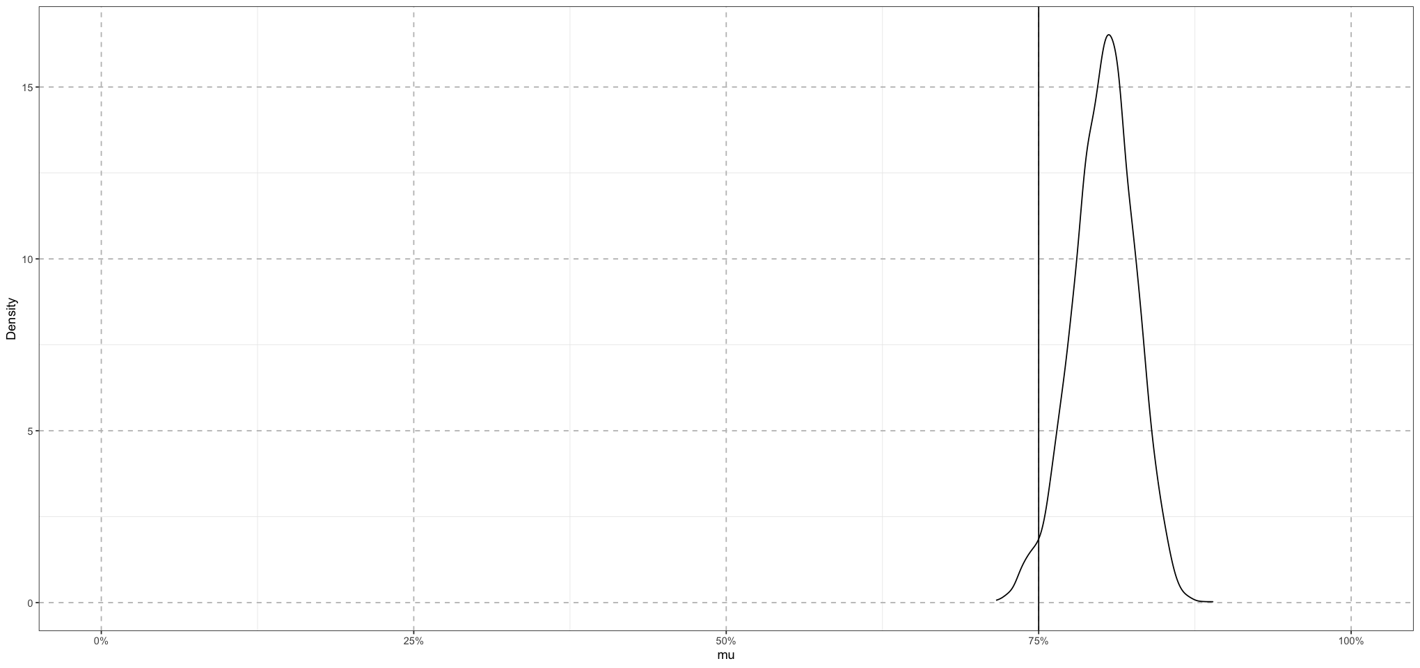
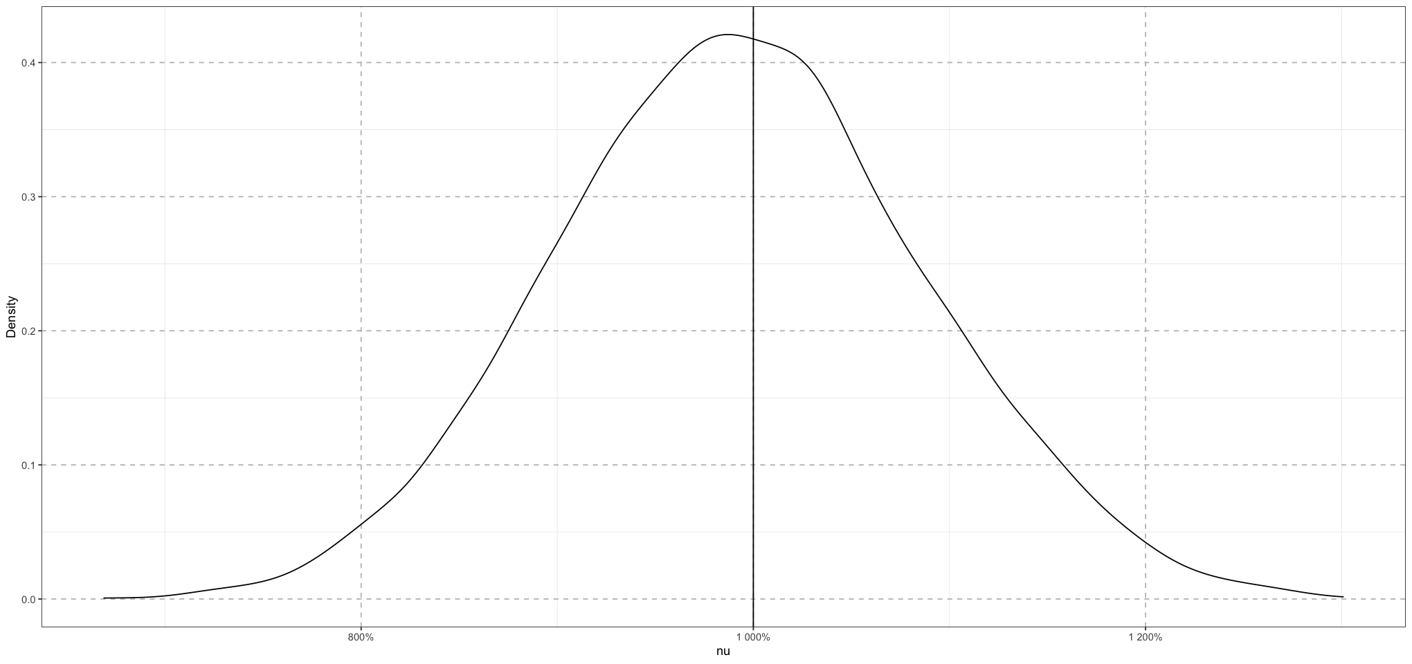
Great! So this model seems to be doing a good job of recovering the actual values. Now that we have some confidence in this part of the model, let’s extend it a bit more to consider the situation of different schools, each with their own means, which now influence the scores of their students. We’ll assume that the schools each draw their means from a single beta distribution, and we’ll also assument that each student draws their score from a beta distribution whose mean is the school mean.
set.seed(1234)
NUM_SCHOOLS <- 5
school_mu <- 0.75
school_nu <- 50

school_alpha <- school_mu * school_nu
school_beta <- (1 - school_mu) * school_nu

school_means <- rbeta(NUM_SCHOOLS, school_alpha, school_beta)

ps <- seq(from = 0, to = 1, length.out = 100)
density <- dbeta(ps, school_alpha, school_beta)
ggplot() +
    geom_line(data = data.frame(p = ps, density = density), mapping = aes(p, density)) +
    geom_point(data = data.frame(p = school_means, density = dbeta(school_means, school_alpha, school_beta)), mapping = aes(p, density)) +
    labs(x = "School-Specific Mean", y = "Density") +
    scale_x_continuous(labels = scales::percent_format(accuracy = 1)) +
    theme_bw() +  # Set background to white
    theme(
        panel.grid.major = element_line(size = 0.5, linetype = 'dashed', colour = "grey"),
    )
Now we’ll simulate some students for each of these schools.
STUDENT_NU <- 30

student_alpha <- school_means * STUDENT_NU
student_beta <- (1 - school_means) * STUDENT_NU

ps <- seq(from = 0, to = 1, length.out = 100)
plot_df <- data.frame(p = numeric(), density = numeric(), school = integer())
for (school_id in 1:NUM_SCHOOLS) {
    alpha <- student_alpha[school_id]
    beta <- student_beta[school_id]
    school_data <- data.frame(
        p = ps,
        density = dbeta(ps, alpha, beta),
        school = school_id
    )
    plot_df <- rbind(plot_df, school_data)
}
plot_df$school <- as.factor(plot_df$school)

ggplot(plot_df, aes(p, density, group = school, colour = school)) +
    geom_line() +
    labs(x = "p", y = 'Density', colour = "School") +
    scale_x_continuous(labels = scales::percent_format(accuracy = 1)) +
    theme_bw() +  # Set background to white
    theme(
        panel.grid.major = element_line(size = 0.5, linetype = 'dashed', colour = "grey"),
    )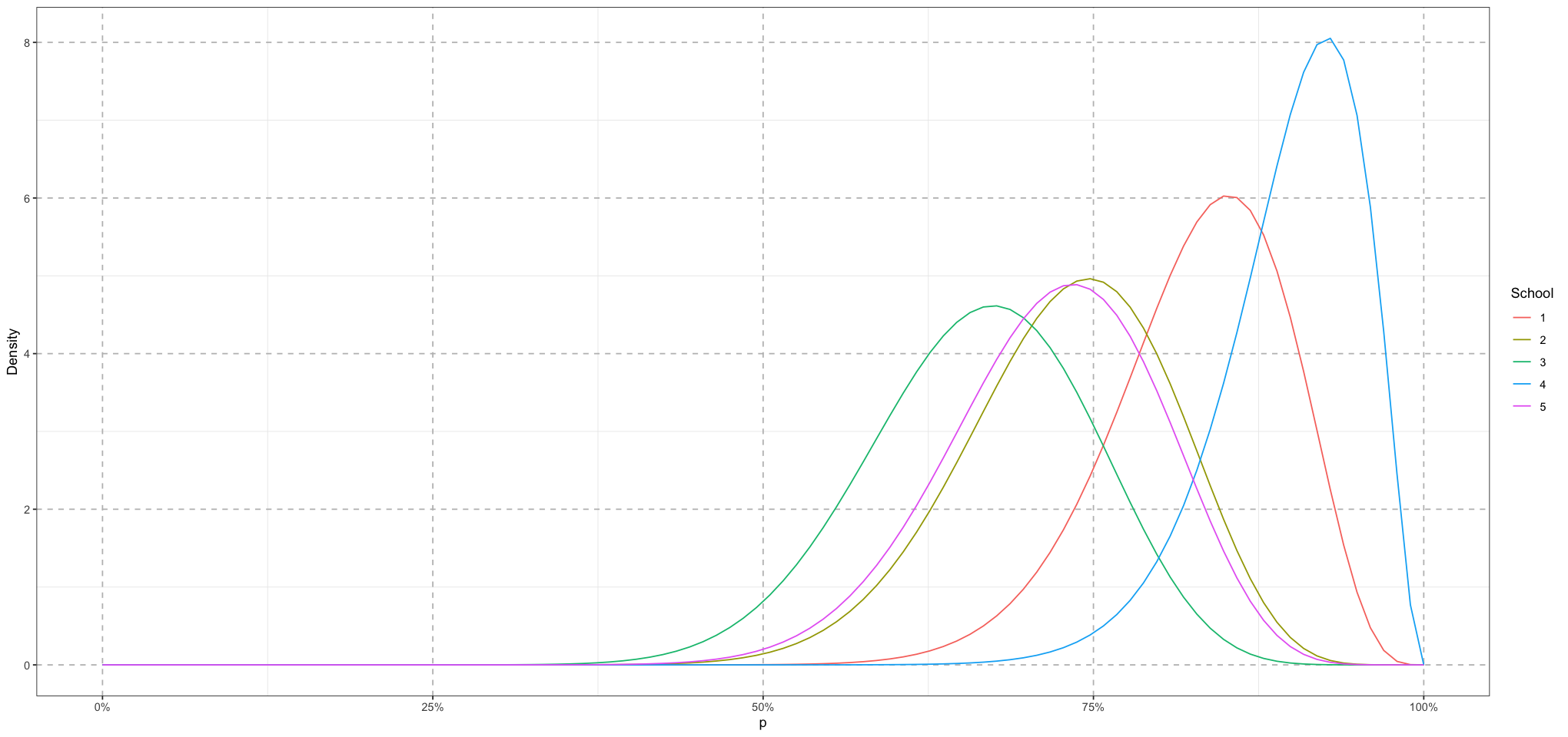
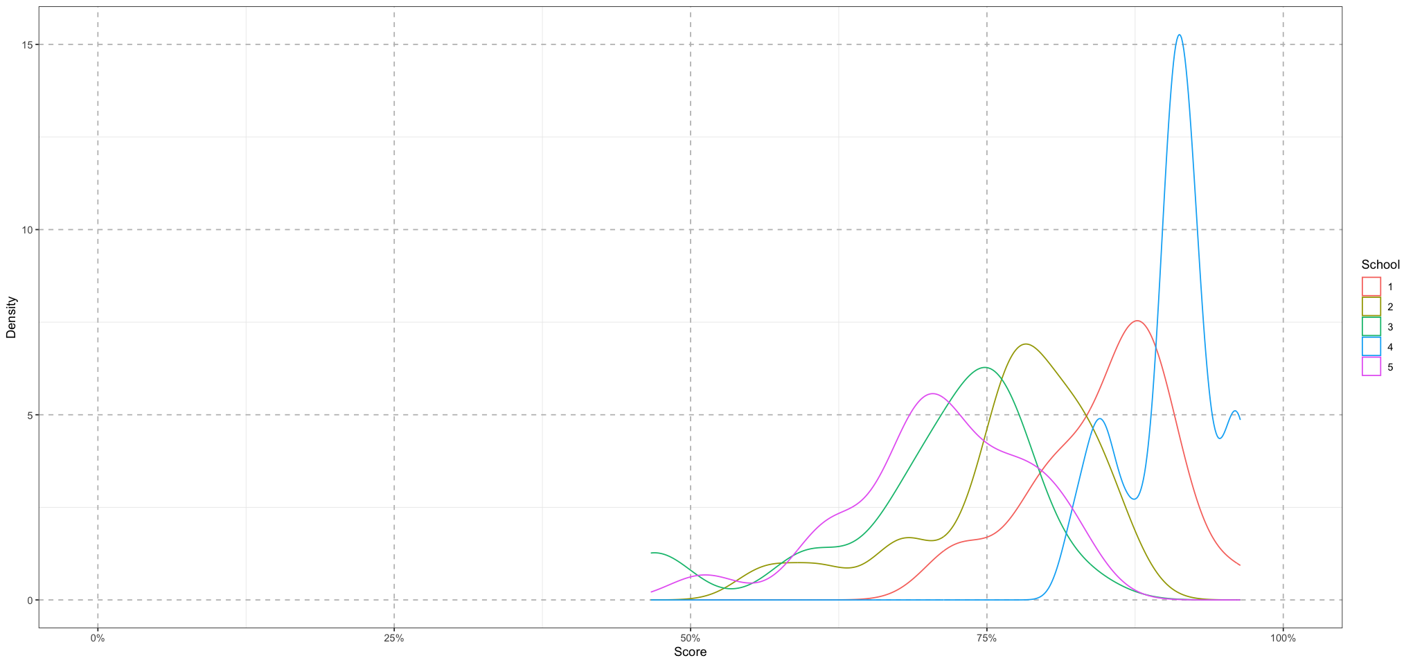
Here we can see the distribution of scores from which each student will draw their scores.
set.seed(1234)
STUDENTS_PER_SCHOOL <- 20
student_scores <- data.frame(s = numeric(), school = integer())

for (school in 1:NUM_SCHOOLS) {
    alpha <- student_alpha[school]
    beta <- student_beta[school]
    school_data <- data.frame(
        s = rbeta(STUDENTS_PER_SCHOOL, alpha, beta),
        school = school
    )
    student_scores <- rbind(student_scores, school_data)
}
student_scores$school <- as.factor(student_scores$school)

ggplot(student_scores, aes(s, colour = school, group = school)) +
    geom_density() +
    coord_cartesian(xlim = c(0, 1)) +
    labs(x = 'Score', y = 'Density', colour = "School") +
    scale_x_continuous(labels = scales::percent_format(accuracy = 1)) +
    theme_bw() +
    theme(
        panel.grid.major = element_line(size = 0.5, linetype = 'dashed', colour = "grey"),
    )
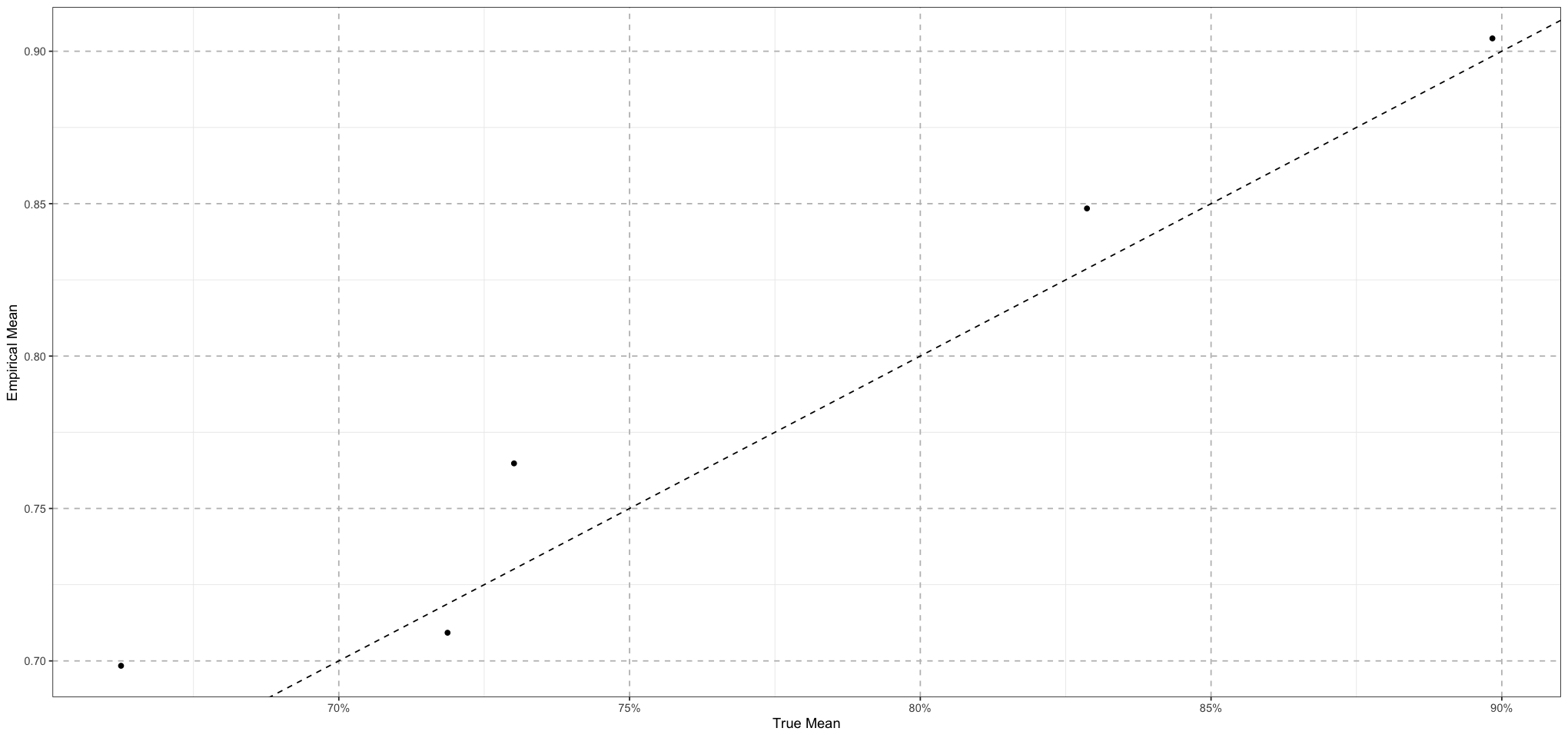
plot_df <- data.frame(true_mean = numeric(), empirical_mean = numeric())
for (school_id in 1:NUM_SCHOOLS) {
    school_data <- student_scores[student_scores$school == school_id, ]
    plot_df <- rbind(plot_df, data.frame(true_mean = school_means[school_id], empirical_mean = mean(school_data$s)))
}

empirical_school_means <- plot_df$empirical_mean

ggplot(plot_df, aes(true_mean, empirical_mean)) +
    geom_point() +
    geom_abline(intercept = 0, slope = 1, linetype = 'dashed') +
    labs(x = "True Mean", y = "Empirical Mean") +
    scale_x_continuous(labels = scales::percent_format(accuracy = 1)) +
    theme_bw() +
    theme(
        panel.grid.major = element_line(size = 0.5, linetype = 'dashed', colour = "grey"),
    )
First, let’s run an unpooled model - that is, one where we estimate each school’s values separately. That model looks like
student_school_unpooled_model_code <- "
data {
    int<lower = 0> N_students; // number of students
    int<lower = 0> N_schools; // number of schools
    vector[N_students] s; // student scores
    array[N_students] int school_id; // the school id for each student
}
parameters {
    array[N_schools] real<lower = 0, upper = 1> mu_school;
    array[N_schools] real<lower = 0> nu_school;
}
 transformed parameters {
    array[N_schools] real<lower = 0> a_school;
    array[N_schools] real<lower = 0> b_school;
    for (i in 1:N_schools) {
        a_school[i] = mu_school[i] * nu_school[i];
        b_school[i] = (1 - mu_school[i]) * nu_school[i];
    }
}
model {
    for (student_index in 1:N_students) {
        s[student_index] ~ beta(a_school[school_id[student_index]], b_school[school_id[student_index]]);
    }
    mu_school ~ beta(3, 1);
    nu_school ~ normal(30, 4);
}
"

student_school_unpooled_model_file <- write_stan_file(student_school_unpooled_model_code)
student_school_unpooled_model <- cmdstan_model(student_school_unpooled_model_file)

student_school_model_data <- list(
    N_students = nrow(student_scores),
    N_schools = NUM_SCHOOLS,
    s = student_scores$s,
    school_id = as.integer(student_scores$school)
)
student_school_unpooled_fit <- student_school_unpooled_model$sample(
    data = student_school_model_data,
    chains = 4
)
student_school_unpooled_fit$summary()
Running MCMC with 4 sequential chains...
All 4 chains finished successfully.
Mean chain execution time: 0.2 seconds.
Total execution time: 0.9 seconds.| variable | mean | median | sd | mad | q5 | q95 | rhat | ess_bulk | ess_tail |
|---|---|---|---|---|---|---|---|---|---|
| <chr> | <dbl> | <dbl> | <dbl> | <dbl> | <dbl> | <dbl> | <dbl> | <dbl> | <dbl> |
| lp__ | 133.2063127 | 133.5330000 | 2.28559835 | 2.11715280 | 128.9039000 | 136.2762000 | 1.0005406 | 1383.865 | 2676.246 |
| mu_school[1] | 0.8466306 | 0.8467865 | 0.01451341 | 0.01407951 | 0.8222164 | 0.8700590 | 1.0012989 | 9296.896 | 2773.345 |
| mu_school[2] | 0.7631883 | 0.7633160 | 0.01666534 | 0.01648503 | 0.7358237 | 0.7897457 | 1.0000816 | 7172.713 | 2855.873 |
| mu_school[3] | 0.6985636 | 0.6984615 | 0.01903218 | 0.01865037 | 0.6669859 | 0.7296387 | 1.0027091 | 7569.557 | 2383.093 |
| mu_school[4] | 0.8986209 | 0.8987715 | 0.01110209 | 0.01102758 | 0.8803896 | 0.9161687 | 1.0006262 | 6881.045 | 2579.987 |
| mu_school[5] | 0.7082870 | 0.7088845 | 0.01838196 | 0.01870893 | 0.6780569 | 0.7377980 | 1.0002342 | 8158.005 | 2954.655 |
| nu_school[1] | 30.5954286 | 30.5384500 | 3.60381506 | 3.63333369 | 24.7442450 | 36.6404500 | 1.0011241 | 6743.832 | 2632.137 |
| nu_school[2] | 30.3578492 | 30.3070000 | 3.71383749 | 3.70813086 | 24.3044150 | 36.6859250 | 1.0022297 | 8089.165 | 2602.090 |
| nu_school[3] | 28.9024282 | 28.8947500 | 3.59228813 | 3.67084347 | 22.9660100 | 34.8531500 | 1.0014781 | 7393.074 | 2979.367 |
| nu_school[4] | 32.0602813 | 32.0718500 | 3.67326279 | 3.72807183 | 26.0406500 | 38.0546350 | 1.0018923 | 7189.690 | 2859.561 |
| nu_school[5] | 30.7457093 | 30.6825500 | 3.78388583 | 3.78374346 | 24.5528400 | 37.0404800 | 1.0004906 | 7702.508 | 2870.507 |
| a_school[1] | 25.9068463 | 25.8534500 | 3.11506217 | 3.11612868 | 20.8941350 | 31.2008100 | 1.0008923 | 6732.695 | 2500.360 |
| a_school[2] | 23.1730379 | 23.1326500 | 2.91251817 | 2.86645884 | 18.5673600 | 28.0946000 | 1.0028086 | 7867.279 | 2794.205 |
| a_school[3] | 20.1909199 | 20.2093000 | 2.57330288 | 2.56801146 | 15.9950150 | 24.4977450 | 1.0010490 | 7449.585 | 2740.689 |
| a_school[4] | 28.8145096 | 28.8517000 | 3.35774104 | 3.36780003 | 23.3074450 | 34.2775750 | 1.0015005 | 7155.198 | 2752.986 |
| a_school[5] | 21.7806440 | 21.6924500 | 2.76944387 | 2.74147566 | 17.2344200 | 26.5064300 | 1.0012976 | 7711.507 | 3129.558 |
| b_school[1] | 4.6885823 | 4.6692700 | 0.68187457 | 0.69292276 | 3.5813565 | 5.8415735 | 0.9999706 | 8123.741 | 2632.944 |
| b_school[2] | 7.1848123 | 7.1599950 | 0.98184417 | 1.00975438 | 5.6196490 | 8.8247815 | 1.0013434 | 8428.792 | 2801.349 |
| b_school[3] | 8.7115083 | 8.6948950 | 1.20813189 | 1.27687442 | 6.7770070 | 10.7226350 | 1.0012211 | 7377.469 | 2786.540 |
| b_school[4] | 3.2457709 | 3.2309500 | 0.48446246 | 0.49350565 | 2.4725655 | 4.0622545 | 1.0008731 | 7247.993 | 2369.960 |
| b_school[5] | 8.9650650 | 8.9528950 | 1.20969315 | 1.20415289 | 6.9710085 | 11.0267150 | 1.0012507 | 7371.608 | 2881.813 |
unpooled_student_school_draws <- as_draws_matrix(student_school_unpooled_fit$draws())# school means
unpooled_school_means_draws <- unpooled_student_school_draws[, grep('mu_school', colnames(unpooled_student_school_draws))]
unpooled_school_mean_means <- apply(unpooled_school_means_draws, 2, mean)
unpooled_school_mean_lower <- apply(unpooled_school_means_draws, 2, function(col) quantile(col, 0.025))
unpooled_school_mean_upper <- apply(unpooled_school_means_draws, 2, function(col) quantile(col, 0.975))
unpooled_means_plot_df <- data.frame(school = 1:NUM_SCHOOLS, mean = unpooled_school_mean_means, lower = unpooled_school_mean_lower, upper = unpooled_school_mean_upper)
unpooled_school_means_plot <- ggplot() +
geom_errorbar(data = unpooled_means_plot_df, mapping = aes(school, ymin = lower, ymax = upper)) +
geom_point(data = unpooled_means_plot_df, aes(school, mean)) +
geom_point(data = data.frame(school = 1:NUM_SCHOOLS, mean = school_means), mapping = aes(school, mean, colour = "True Mean")) +
geom_point(data = data.frame(school = 1:NUM_SCHOOLS, mean = empirical_school_means), mapping = aes(school, mean, colour = 'Empirical Mean')) +
labs(x = "School", y = "Mean Score", colour = "Type") +
scale_y_continuous(labels = scales::percent_format(accuracy = 1)) +
theme_bw() +
theme(
panel.grid.major = element_line(size = 0.5, linetype = 'dashed', colour = "grey"),
)
print(unpooled_school_means_plot)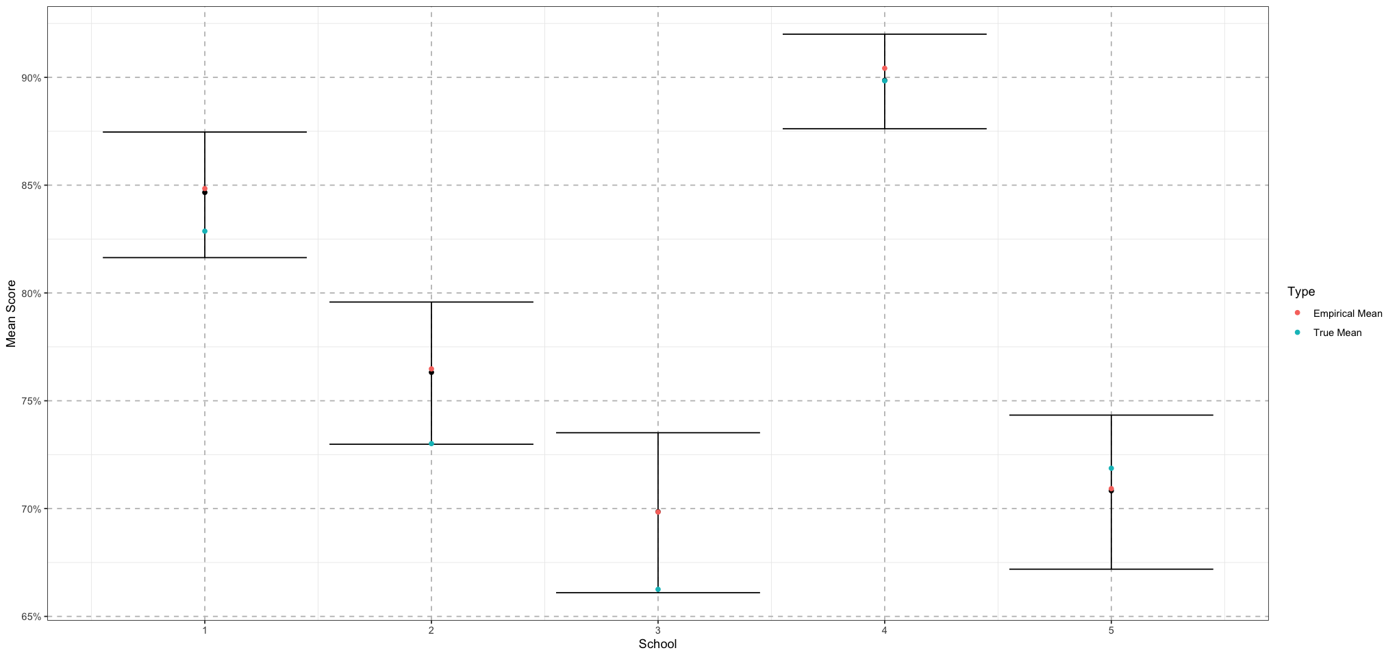
This looks pretty good! We’re doing a good job of recovering these values. Now let’s share information among the schools by using a hierarchical model.
We’ll use the following model to recover the values.
student_school_model_code <- "
data {
    int<lower = 0> N_students; // number of students
    int<lower = 0> N_schools; // number of schools
    vector[N_students] s; // student scores
    array[N_students] int school_id; // the school id for each student
}
parameters {
    array[N_schools] real<lower = 0, upper = 1> mu_school;
    array[N_schools] real<lower = 0> nu_school_raw; // non-centred parameterization; implies nu_school ~ normal(nu_bar, sigma_bar)
    real<lower = 0> alpha_bar;
    real<lower = 0> beta_bar;
    real<lower = 0> nu_bar;
    real<lower = 0> sigma_nu;
}
 transformed parameters {
    array[N_schools] real<lower = 0> nu_school;
    array[N_schools] real<lower = 0> a_school;
    array[N_schools] real<lower = 0> b_school;
    for (i in 1:N_schools) {
        nu_school[i] = nu_bar + sigma_nu * nu_school_raw[i];
        a_school[i] = mu_school[i] * nu_school[i];
        b_school[i] = (1 - mu_school[i]) * nu_school[i];
    }
}
model {
    for (student_index in 1:N_students) {
        s[student_index] ~ beta(a_school[school_id[student_index]], b_school[school_id[student_index]]);
    }
    mu_school ~ beta(alpha_bar, beta_bar);
    nu_school_raw ~ std_normal();
    alpha_bar ~ normal(3, 0.5);
    beta_bar ~ normal(1, 0.3);
    nu_bar ~ normal(30, 5);
    sigma_nu ~ exponential(1);
}
"

student_school_model_file <- write_stan_file(student_school_model_code)
student_school_model <- cmdstan_model(student_school_model_file)

student_school_fit <- student_school_model$sample(
    data = student_school_model_data,
    chains = 4,
    iter_warmup = 1000,
    adapt_delta = 0.95
)
student_school_fit$summary()
Running MCMC with 4 sequential chains...
All 4 chains finished successfully.
Mean chain execution time: 0.4 seconds.
Total execution time: 1.9 seconds.| variable | mean | median | sd | mad | q5 | q95 | rhat | ess_bulk | ess_tail |
|---|---|---|---|---|---|---|---|---|---|
| <chr> | <dbl> | <dbl> | <dbl> | <dbl> | <dbl> | <dbl> | <dbl> | <dbl> | <dbl> |
| lp__ | 120.2997945 | 120.6395000 | 2.88945094 | 2.76875550 | 114.91420000 | 124.4150000 | 1.0048682 | 1490.839 | 2390.733 |
| mu_school[1] | 0.8470211 | 0.8472085 | 0.01358558 | 0.01298165 | 0.82471955 | 0.8688271 | 1.0010532 | 5050.164 | 2470.032 |
| mu_school[2] | 0.7638199 | 0.7639385 | 0.01594188 | 0.01603803 | 0.73703180 | 0.7900103 | 1.0010624 | 5844.673 | 3214.262 |
| mu_school[3] | 0.6989982 | 0.6991170 | 0.01758573 | 0.01766592 | 0.67012455 | 0.7275320 | 1.0017414 | 5188.370 | 3085.584 |
| mu_school[4] | 0.8983489 | 0.8985485 | 0.01102625 | 0.01115063 | 0.88029595 | 0.9159538 | 1.0025573 | 5146.175 | 3025.248 |
| mu_school[5] | 0.7082870 | 0.7083660 | 0.01716313 | 0.01705657 | 0.67989185 | 0.7368971 | 0.9997209 | 5376.621 | 3100.150 |
| nu_school_raw[1] | 0.8128569 | 0.6926650 | 0.61102128 | 0.60914400 | 0.07260510 | 1.9961565 | 1.0004995 | 3516.625 | 1721.888 |
| nu_school_raw[2] | 0.7895747 | 0.6723220 | 0.60165921 | 0.59760344 | 0.05733236 | 1.9660335 | 1.0005797 | 3220.242 | 1853.584 |
| nu_school_raw[3] | 0.7553973 | 0.6324210 | 0.58797066 | 0.56209072 | 0.05570231 | 1.9002925 | 1.0004686 | 2797.938 | 1643.460 |
| nu_school_raw[4] | 0.8333840 | 0.7106100 | 0.62189482 | 0.62426430 | 0.05943881 | 2.0247330 | 0.9998461 | 2781.631 | 1139.225 |
| nu_school_raw[5] | 0.8048431 | 0.6786530 | 0.61165042 | 0.60419731 | 0.06066773 | 2.0173890 | 1.0009278 | 2768.546 | 1470.845 |
| alpha_bar | 3.1320128 | 3.1337150 | 0.46785786 | 0.47165954 | 2.35937800 | 3.8970855 | 1.0019146 | 5119.352 | 2751.850 |
| beta_bar | 1.0907279 | 1.0844350 | 0.24464134 | 0.24603302 | 0.69713060 | 1.5043975 | 1.0009313 | 5496.958 | 2344.933 |
| nu_bar | 31.5787906 | 31.5582500 | 3.37920085 | 3.41346411 | 26.21277500 | 37.1670300 | 1.0003554 | 4995.001 | 3090.744 |
| sigma_nu | 1.0272002 | 0.7143280 | 1.02022647 | 0.73669653 | 0.05808706 | 3.0601565 | 1.0002520 | 4038.993 | 2059.170 |
| nu_school[1] | 32.4157204 | 32.3271500 | 3.43742095 | 3.45297540 | 26.91420000 | 38.1362350 | 1.0009389 | 4991.626 | 3188.874 |
| nu_school[2] | 32.3700213 | 32.2914000 | 3.43706176 | 3.44141112 | 26.87087000 | 38.0587250 | 1.0006216 | 5166.621 | 3033.495 |
| nu_school[3] | 32.3245989 | 32.2764500 | 3.42172188 | 3.45601473 | 26.84857000 | 38.0114750 | 1.0005946 | 5223.580 | 3131.844 |
| nu_school[4] | 32.4816132 | 32.4246500 | 3.47454623 | 3.44066982 | 26.96652500 | 38.3314700 | 1.0007982 | 5070.896 | 3205.803 |
| nu_school[5] | 32.3932509 | 32.2758500 | 3.43845039 | 3.44600718 | 26.99057000 | 38.1477100 | 1.0007019 | 5338.495 | 3007.364 |
| a_school[1] | 27.4618737 | 27.3681500 | 2.99122402 | 2.98136034 | 22.71480500 | 32.3846850 | 1.0005317 | 4961.919 | 3132.647 |
| a_school[2] | 24.7285854 | 24.6540000 | 2.70788908 | 2.68691598 | 20.37299000 | 29.2811650 | 1.0002278 | 5146.804 | 3083.624 |
| a_school[3] | 22.5988739 | 22.5553500 | 2.49258392 | 2.49840339 | 18.63084000 | 26.8150650 | 1.0001400 | 5127.857 | 3115.493 |
| a_school[4] | 29.1838142 | 29.0871500 | 3.17859264 | 3.14333439 | 24.18315500 | 34.4842300 | 1.0010808 | 4943.275 | 3131.463 |
| a_school[5] | 22.9453409 | 22.8683500 | 2.51432791 | 2.52901908 | 19.04795500 | 27.2467150 | 1.0001032 | 5396.115 | 3104.879 |
| b_school[1] | 4.9538464 | 4.9310000 | 0.64619137 | 0.64508667 | 3.93117700 | 6.0525920 | 1.0019177 | 5480.992 | 3080.917 |
| b_school[2] | 7.6414370 | 7.6174150 | 0.93165746 | 0.91027192 | 6.15480500 | 9.2250720 | 1.0012027 | 5484.039 | 3014.747 |
| b_school[3] | 9.7257252 | 9.6761700 | 1.14435871 | 1.16653192 | 7.94368300 | 11.6919750 | 1.0018870 | 5549.259 | 2891.207 |
| b_school[4] | 3.2977995 | 3.2701050 | 0.47490024 | 0.46661129 | 2.53166850 | 4.1071670 | 1.0008953 | 5902.171 | 2746.835 |
| b_school[5] | 9.4479103 | 9.4035900 | 1.13083864 | 1.13598295 | 7.68017550 | 11.3531550 | 1.0005881 | 5082.952 | 3188.104 |
student_school_draws <- as_draws_matrix(student_school_fit$draws())# # school means
school_means_draws <- student_school_draws[, grep('mu_school', colnames(student_school_draws))]
school_mean_means <- apply(school_means_draws, 2, mean)
school_mean_lower <- apply(school_means_draws, 2, function(col) quantile(col, 0.025))
school_mean_upper <- apply(school_means_draws, 2, function(col) quantile(col, 0.975))
means_plot_df <- data.frame(school = 1:NUM_SCHOOLS, mean = school_mean_means, lower = school_mean_lower, upper = school_mean_upper)
prior_mean <- mean(student_school_draws[, 'alpha_bar'] / (student_school_draws[, 'alpha_bar'] + student_school_draws[, 'beta_bar']))
pooled_school_means_plot <- ggplot() +
geom_errorbar(data = means_plot_df, mapping = aes(school, ymin = lower, ymax = upper)) +
geom_point(data = means_plot_df, aes(school, mean)) +
geom_point(data = data.frame(school = 1:NUM_SCHOOLS, mean = school_means), mapping = aes(school, mean, colour = 'True Mean')) +
geom_point(data = data.frame(school = 1:NUM_SCHOOLS, mean = unpooled_school_mean_means), aes(school, mean, colour = "Unpooled Mean")) +
geom_hline(mapping = aes(yintercept = prior_mean), linetype = 'dashed') +
labs(x = "School", y = "Value", colour = "Mean Type") +
scale_y_continuous(labels = scales::percent_format(accuracy = 1)) +
theme_bw() +
theme(
panel.grid.major = element_line(size = 0.5, linetype = 'dashed', colour = "grey"),
)
print(pooled_school_means_plot)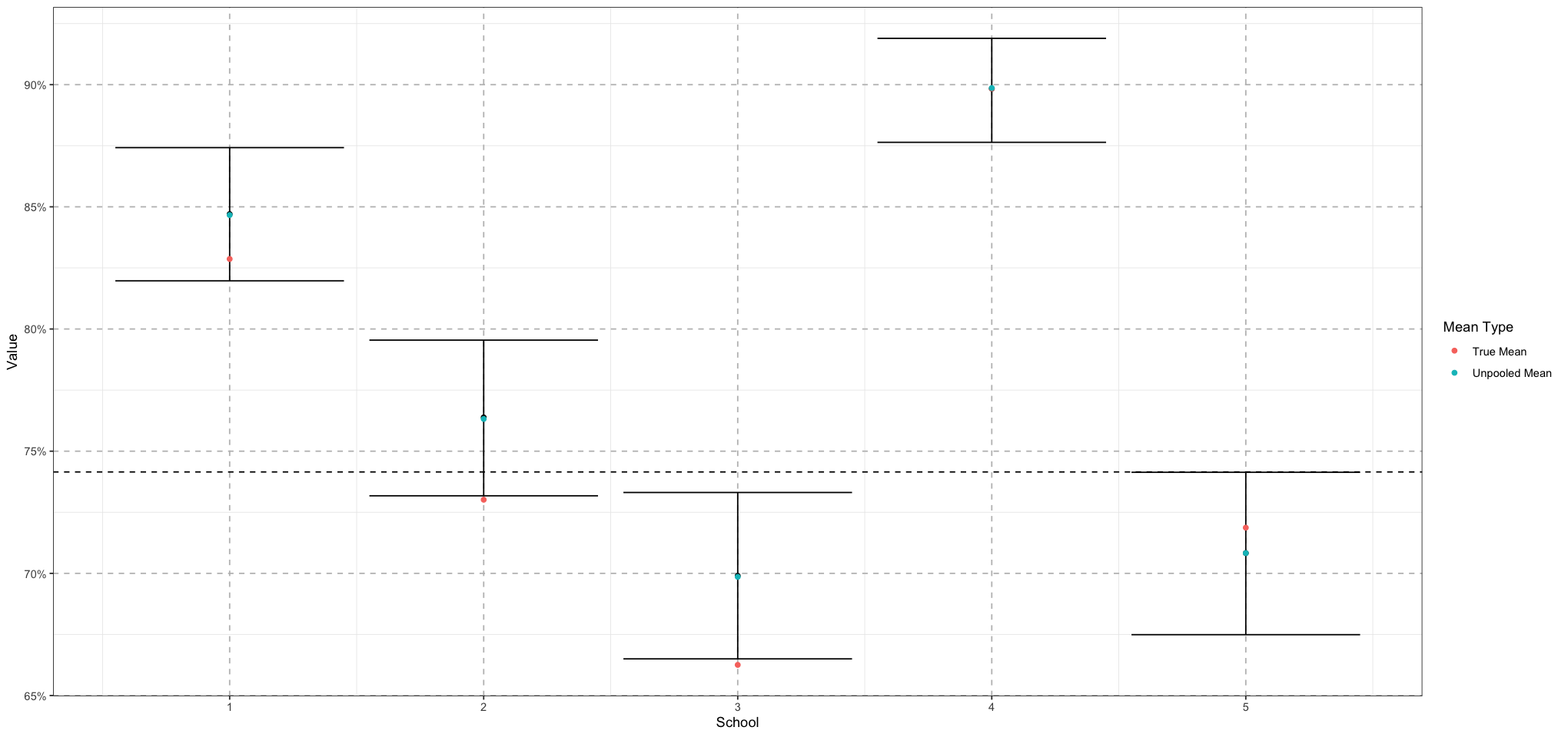
So as we can see, pooling didn’t have too much of an effect; there’s a minimal change from the pooled mean (black) and the unpooled mean (blue).
Now we’re ready to tackle a more complex hierarchical model with multiple layers! To start off, let’s say we have some districts. Each district will have some schools, and each school will have some students. Each of the students will have a score that is the school mean plus some standard deviation, drawn from a beta distribution. In turn, each of the school means for a district will be drawn from the same distribution. Finally, each of the district means will be drawn from a different shared distribution.
set.seed(1234)

NUM_DISTRICTS <- 3
SCHOOLS_PER_DISTRICT <- 3
TOTAL_SCHOOLS <- NUM_DISTRICTS * SCHOOLS_PER_DISTRICT
STUDENTS_PER_SCHOOL <- 20
TOTAL_STUDENTS <- TOTAL_SCHOOLS * STUDENTS_PER_SCHOOL

district_mu <- 0.75
district_nu <- 30
district_alpha <- district_mu * district_nu
district_beta <- (1 - district_mu) * district_nu

district_means <- rbeta(NUM_DISTRICTS, district_alpha, district_beta)
ps <- seq(from = 0, to = 1, length.out = 100)
district_distribution_df <- data.frame(
    p = ps,
    density = dbeta(ps, district_alpha, district_beta)
)
districts_df <- data.frame(
    p = district_means,
    density = dbeta(district_means, district_alpha, district_beta)
)
ggplot(NULL, aes(p, density)) +
    geom_line(data = district_distribution_df) +
    geom_point(data = districts_df) +
    labs(x = "p", y = "Density") +
    scale_x_continuous(labels = scales::percent_format(accuracy = 1)) +
    theme_bw() +
    theme(
        panel.grid.major = element_line(size = 0.5, linetype = 'dashed', colour = "grey"),
    )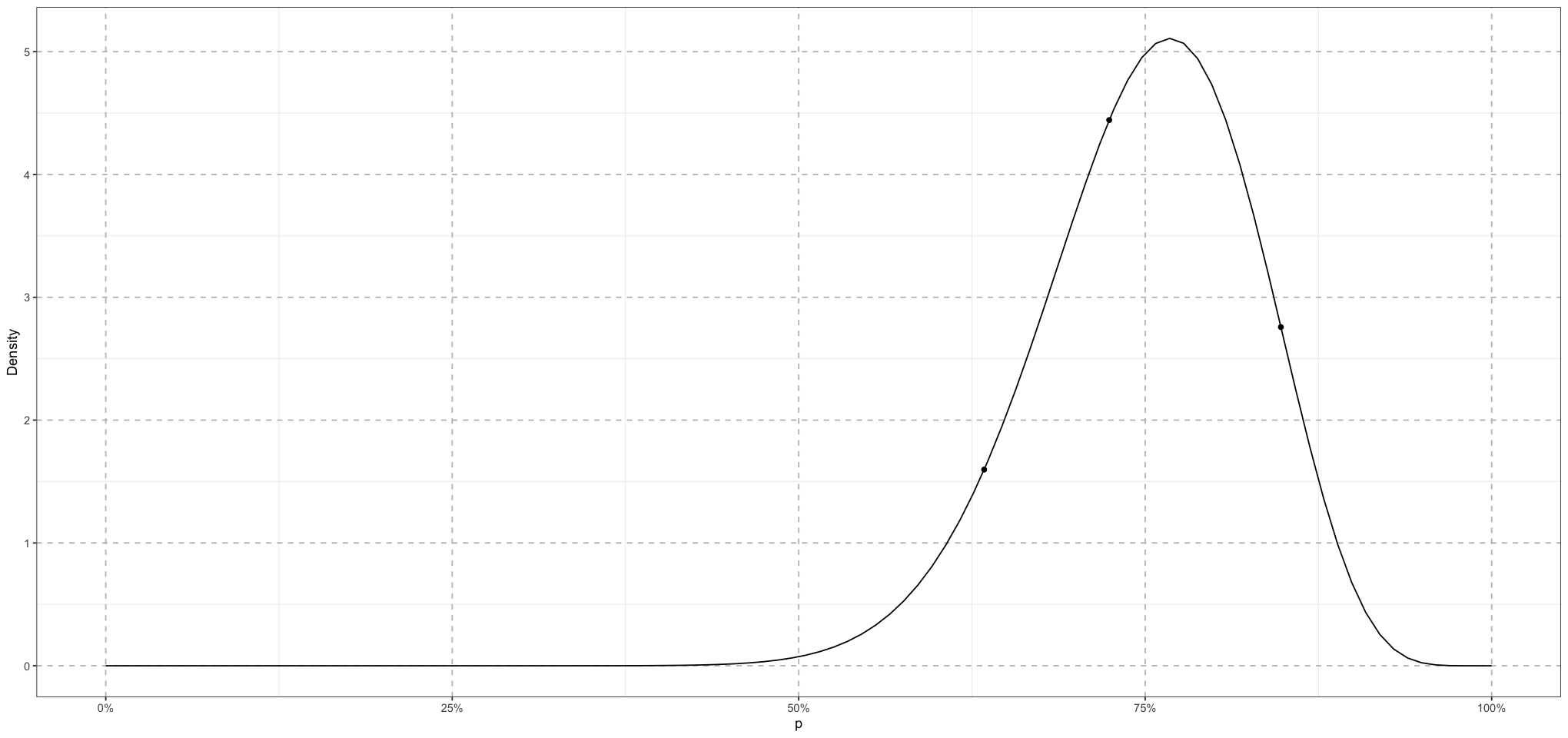
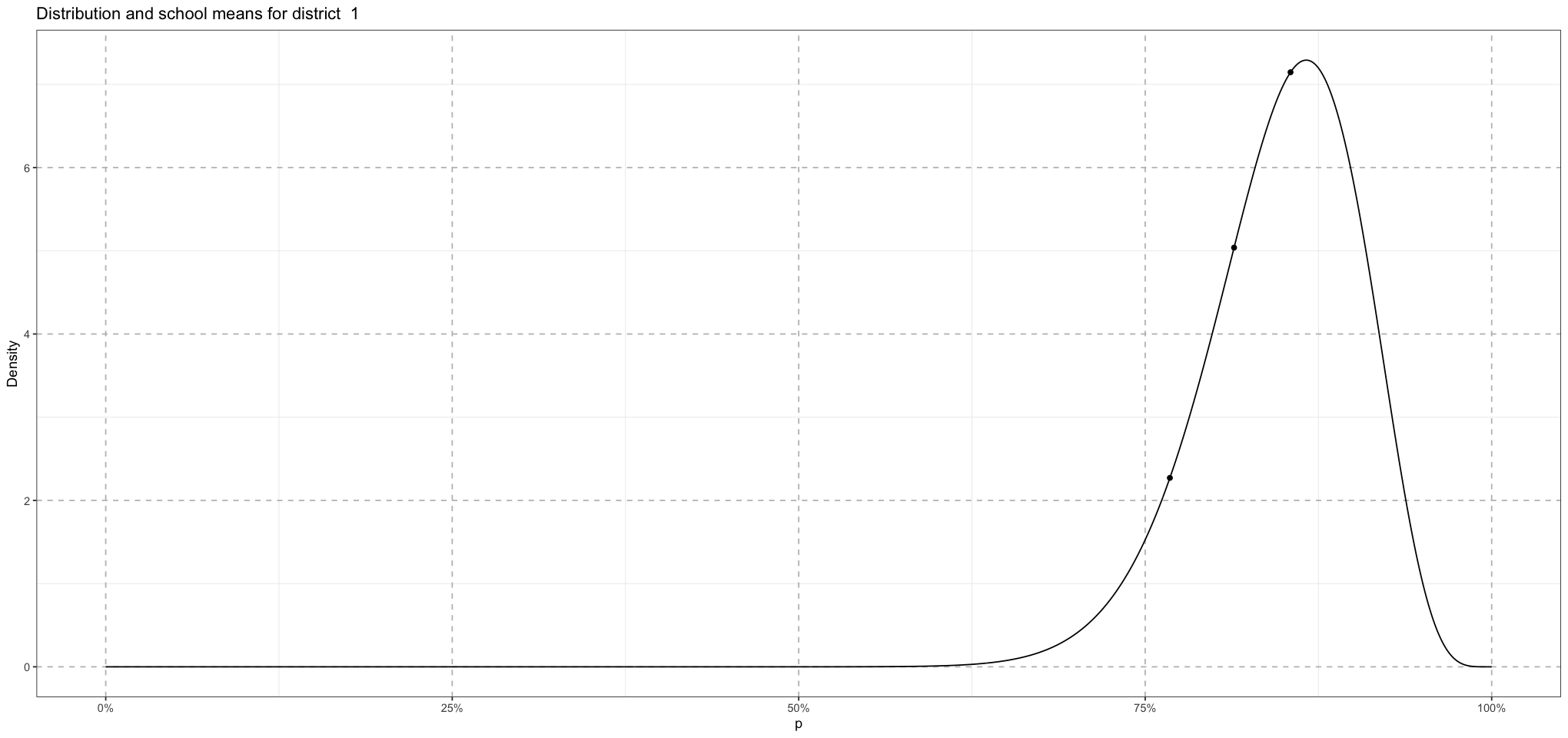
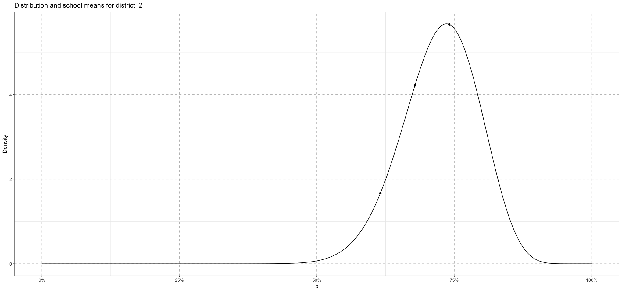
So now we have the district means coming from a single distribution. Within that, each district will have schools, each of whose means comes from a distribution whose mean is the district mean!
set.seed(2024)
ps <- seq(from = 0, to = 1, length.out = 1e3)
school_params <- data.frame(district = integer(), school_id = integer(), school_mu = numeric())
district_nu <- 40
for (district_id in 1:NUM_DISTRICTS) {
    district_mu <- district_means[district_id]
    district_alpha <- district_mu * district_nu
    district_beta <- (1 - district_mu) * district_nu
    school_data <- data.frame(
        district = rep(district_id, SCHOOLS_PER_DISTRICT),
        school_id = district_id + 1:SCHOOLS_PER_DISTRICT,
        school_mu = rbeta(SCHOOLS_PER_DISTRICT, district_alpha, district_beta)
    )
    school_params <- rbind(school_params, school_data)

    district_distribution_df <- data.frame(p = ps, density = dbeta(ps, district_alpha, district_beta))
    school_means_df <- data.frame(p = school_data$school_mu, density = dbeta(school_data$school_mu, district_alpha, district_beta))
    school_plot <- ggplot(NULL, aes(p, density)) +
        geom_line(data = district_distribution_df) +
        geom_point(data = school_means_df) +
        labs(x = "p", y = "Density", title = paste("Distribution and school means for district ", district_id)) +
        scale_x_continuous(labels = scales::percent_format(accuracy = 1)) +
        theme_bw() +
        theme(
            panel.grid.major = element_line(size = 0.5, linetype = 'dashed', colour = "grey"),
        )
    print(school_plot)
}
Now that we have the school information, we can generate a simulated group of students for each school. Each student will draw their score from a distribution whose mean is the school mean.
set.seed(2024)
ps <- seq(from = 0, to = 1, length.out = 1e3)
student_data <- data.frame(district_id = integer(), school_id = integer(), score = numeric())
student_nu <- 30
for (school_id in 1:TOTAL_SCHOOLS) {
    district_id <- school_params[school_id, 'district']
    school_mu <- school_params[school_id, 'school_mu']
    student_alpha <- school_mu * student_nu
    student_beta <- (1 - school_mu) * student_nu
    school_scores <- data.frame(
        district_id = rep(district_id, STUDENTS_PER_SCHOOL),
        school_id <- rep(school_id, STUDENTS_PER_SCHOOL),
        score = rbeta(STUDENTS_PER_SCHOOL, student_alpha, student_beta)
    )
    student_data <- rbind(student_data, school_scores)
}
student_data$student_id <- as.factor(seq_len(nrow(student_data)))
student_data$school_id <- as.factor(student_data$school_id)
student_data$district_id <- as.factor(student_data$district_id)

student_plot <- ggplot(student_data, aes(student_id, score)) +
    geom_point(aes(colour = school_id, shape = district_id)) +
    labs(x = "Student", y = "Score", colour = "School", shape = "District") +
    scale_y_continuous(labels = scales::percent_format(accuracy = 1)) +
    theme_bw() +  # Set background to white
    theme(
        panel.grid.major.x = element_blank(),
        panel.grid.minor.x = element_blank(),
        panel.grid.major.y = element_line(size = 0.5, linetype = 'dashed', colour = "grey"),
        axis.ticks.x = element_blank(),
        axis.text.x = element_blank(),
    )
for (district_id in 1:(NUM_DISTRICTS - 1)) {
    print(district_id)
    student_plot <- student_plot +
        geom_vline(xintercept = SCHOOLS_PER_DISTRICT * STUDENTS_PER_SCHOOL * district_id + 0.5)
}
print(student_plot)
[1] 1
[1] 2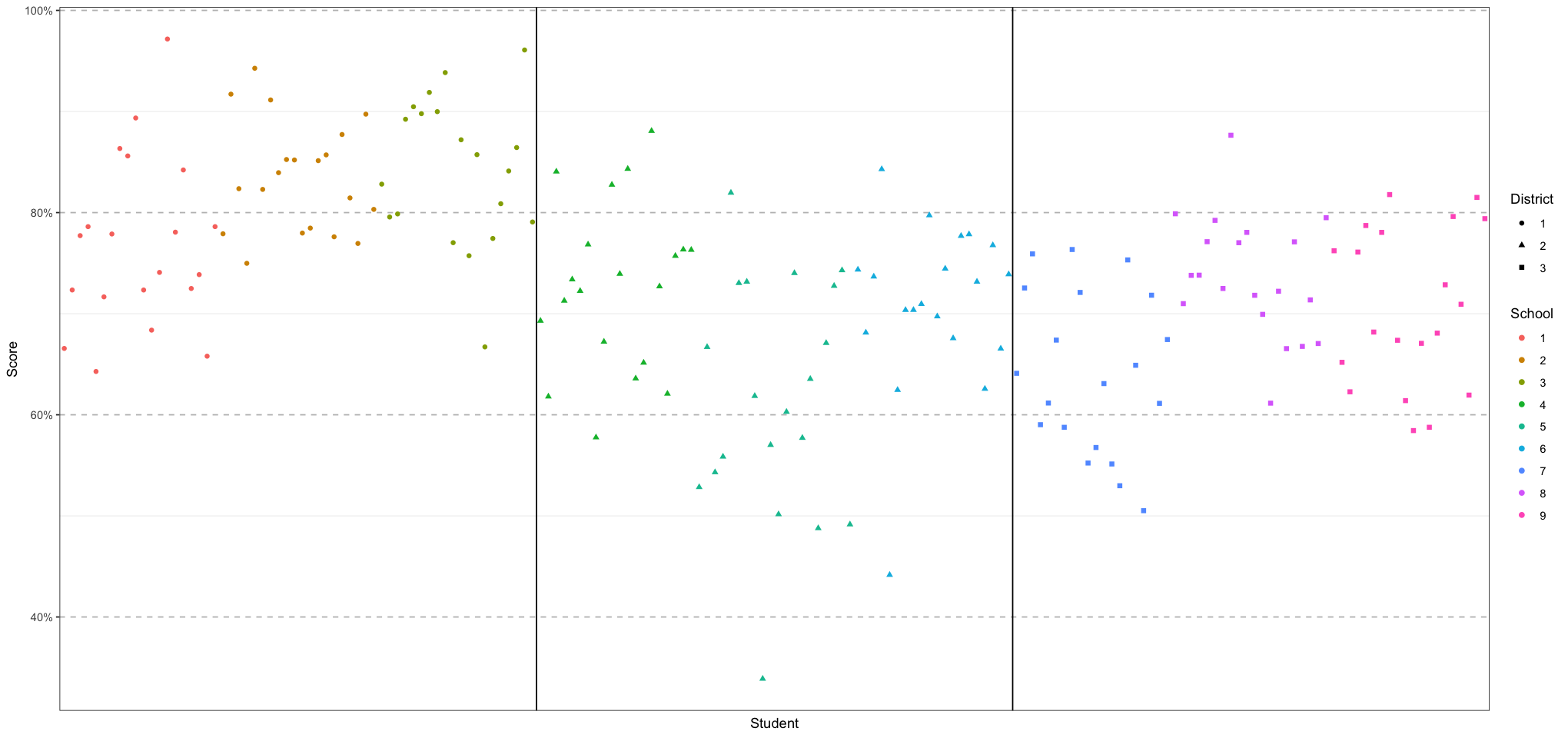
Great! Now that we have the data and a good handle on the generation process, let’s look what this looks like as a model. Again, there are a few levels here. There will be a shared district-level set of parameters as well as a shared school-level set of parameters influenced by the district. The student will in turn have their own parameters, again inheriting from the school parameters. There’s a lot here, but let’s see what it looks like in Stan!
# NB: this is the non-centred parameterization to avoid divergent transitions
student_school_district_model_code <- "
data {
    int<lower = 0> N_students; // number of students
    int<lower = 0> N_schools; // number of schools
    int<lower = 0> N_districts; // number of districts
    vector[N_students] s; // student scores
    array[N_students] int school_id; // the school id for each student
    array[N_schools] int district_id; // the district for each school
}
parameters {
    array[N_districts] real<lower = 0, upper = 1> mu_district;
    array[N_districts] real<lower = 0> nu_district_raw; // standard normal -> implies nu_school ~ normal(nu_bar, sigma_nu)
    array[N_schools] real<lower = 0, upper = 1> mu_school;
    array[N_schools] real<lower = 0> nu_school;
    real<lower = 0> alpha_bar;
    real<lower = 0> beta_bar;
    real<lower = 0> nu_bar;
    real<lower = 0> sigma_nu;
}
 transformed parameters {
    // array[N_schools] real<lower = 0> nu_school;
    array[N_schools] real<lower = 0> a_school;
    array[N_schools] real<lower = 0> b_school;
    array[N_districts] real<lower = 0> a_district;
    array[N_districts] real <lower = 0> b_district;
    array[N_districts] real <lower = 0> nu_district;
    for (i in 1:N_schools) {
        // nu_school[i] = nu_bar + sigma_nu * nu_school_raw[i];
        a_school[i] = mu_school[i] * nu_school[i];
        b_school[i] = (1 - mu_school[i]) * nu_school[i];
    }
    for (district_index in 1:N_districts) {
        nu_district[district_index] = nu_bar + sigma_nu * nu_district_raw[district_index];
        a_district[district_index] = mu_district[district_index] * nu_district[district_index];
        b_district[district_index] = (1 - mu_district[district_index]) * nu_district[district_index];
    }
}
model {
    for (student_index in 1:N_students) {
        s[student_index] ~ beta(a_school[school_id[student_index]], b_school[school_id[student_index]]);
    }
    for (school_index in 1:N_schools) {
        mu_school[school_index] ~ beta(a_district[district_id[school_index]], b_district[district_id[school_index]]);
    }
    mu_district ~ beta(alpha_bar, beta_bar);
    nu_district_raw ~ std_normal();

    // hyperpriors
    alpha_bar ~ normal(3, 0.5);
    beta_bar ~ normal(1, 0.3);
    nu_bar ~ normal(40, 5);
    sigma_nu ~ exponential(1);
}
"

student_school_district_model_file <- write_stan_file(student_school_district_model_code)
student_school_district_model <- cmdstan_model(student_school_district_model_file)

student_school_district_model_data <- list(
    N_students = nrow(student_data),
    N_schools = length(unique(student_data$school_id)),
    N_districts = length(unique(student_data$district_id)),
    s = student_data$score,
    school_id = student_data$school_id,
    district_id = school_params$district
)

student_school_district_fit <- student_school_district_model$sample(
    data = student_school_district_model_data,
    chains = 4,
    iter_warmup = 1000,
    adapt_delta = 0.95
)
student_school_district_fit$summary()
Running MCMC with 4 sequential chains...
All 4 chains finished successfully.
Mean chain execution time: 0.9 seconds.
Total execution time: 3.9 seconds.| variable | mean | median | sd | mad | q5 | q95 | rhat | ess_bulk | ess_tail |
|---|---|---|---|---|---|---|---|---|---|
| <chr> | <dbl> | <dbl> | <dbl> | <dbl> | <dbl> | <dbl> | <dbl> | <dbl> | <dbl> |
| lp__ | 222.7176947 | 223.0595000 | 3.93686660 | 3.79693860 | 215.76725000 | 228.5353500 | 1.0035301 | 1654.261 | 2357.782 |
| mu_district[1] | 0.8108640 | 0.8118355 | 0.03423787 | 0.03307384 | 0.75313205 | 0.8667575 | 1.0005594 | 5053.485 | 2857.642 |
| mu_district[2] | 0.6840614 | 0.6850335 | 0.04265020 | 0.04337569 | 0.61480330 | 0.7528840 | 1.0017076 | 3930.215 | 2879.500 |
| mu_district[3] | 0.6941475 | 0.6959630 | 0.04198568 | 0.04179153 | 0.62348970 | 0.7613662 | 1.0008498 | 5018.537 | 2966.480 |
| nu_district_raw[1] | 0.8080386 | 0.6769430 | 0.60914963 | 0.60004825 | 0.06027230 | 1.9802930 | 0.9999384 | 3687.749 | 1631.689 |
| nu_district_raw[2] | 0.7951544 | 0.6724660 | 0.59759151 | 0.58762851 | 0.06592412 | 1.9247665 | 1.0015042 | 2791.602 | 1709.045 |
| nu_district_raw[3] | 0.8103433 | 0.6857005 | 0.60298377 | 0.59143509 | 0.06953199 | 1.9685580 | 1.0001191 | 3552.671 | 1907.645 |
| mu_school[1] | 0.7745501 | 0.7750630 | 0.02028668 | 0.01939241 | 0.73972350 | 0.8062264 | 1.0015966 | 4542.343 | 2547.013 |
| mu_school[2] | 0.8342911 | 0.8349070 | 0.01277099 | 0.01272219 | 0.81273770 | 0.8545590 | 1.0011919 | 4220.755 | 3036.484 |
| mu_school[3] | 0.8395642 | 0.8404945 | 0.01672362 | 0.01640942 | 0.81096990 | 0.8656431 | 1.0010039 | 4468.803 | 2866.154 |
| mu_school[4] | 0.7244529 | 0.7250115 | 0.01776163 | 0.01737237 | 0.69428420 | 0.7529640 | 1.0009774 | 3779.505 | 2623.897 |
| mu_school[5] | 0.6209195 | 0.6212540 | 0.02417814 | 0.02367193 | 0.58176280 | 0.6599121 | 1.0006665 | 4574.196 | 2910.079 |
| mu_school[6] | 0.7070876 | 0.7075630 | 0.01730462 | 0.01654804 | 0.67776680 | 0.7344344 | 0.9997740 | 4020.686 | 2711.795 |
| mu_school[7] | 0.6434111 | 0.6434790 | 0.01701471 | 0.01667184 | 0.61544455 | 0.6715378 | 1.0011385 | 4227.745 | 2632.624 |
| mu_school[8] | 0.7353718 | 0.7358175 | 0.01382481 | 0.01381042 | 0.71246380 | 0.7575197 | 1.0012051 | 3897.445 | 2490.404 |
| mu_school[9] | 0.7056546 | 0.7066625 | 0.01718360 | 0.01605433 | 0.67772540 | 0.7324504 | 1.0004752 | 4186.585 | 2553.651 |
| nu_school[1] | 19.2145683 | 18.5469500 | 5.71679088 | 5.46189840 | 11.00878000 | 29.4999550 | 0.9997007 | 4618.797 | 2857.748 |
| nu_school[2] | 43.2529643 | 41.9769500 | 13.32993696 | 12.86148087 | 24.15926000 | 67.6573800 | 1.0001604 | 4144.801 | 2702.517 |
| nu_school[3] | 25.7384937 | 24.9508000 | 7.72034944 | 7.77319767 | 14.41916500 | 39.5445250 | 1.0004349 | 3992.273 | 3020.537 |
| nu_school[4] | 30.0836856 | 29.1282000 | 9.12058981 | 8.83051386 | 16.85719500 | 46.4470350 | 1.0002684 | 4392.158 | 2939.064 |
| nu_school[5] | 18.6909772 | 18.1623000 | 5.52931243 | 5.42742795 | 10.69125500 | 28.4436700 | 1.0003793 | 4818.263 | 3010.402 |
| nu_school[6] | 34.3268246 | 33.3853000 | 10.33198302 | 9.93253044 | 19.77090500 | 52.8546050 | 1.0001168 | 4400.425 | 2784.537 |
| nu_school[7] | 38.6659344 | 37.6974000 | 11.69556233 | 11.55316050 | 21.88963000 | 59.5734650 | 1.0024960 | 5346.653 | 2871.480 |
| nu_school[8] | 55.3977254 | 53.8983000 | 17.19780834 | 16.83129063 | 30.63416500 | 86.0647300 | 1.0006023 | 4799.014 | 3115.822 |
| nu_school[9] | 36.4689579 | 35.2106500 | 11.43582314 | 11.03187834 | 20.13321000 | 57.4454050 | 1.0001742 | 4279.718 | 2810.782 |
| alpha_bar | 3.0422431 | 3.0382050 | 0.48231749 | 0.47995469 | 2.24597800 | 3.8459800 | 0.9999978 | 5304.740 | 2262.935 |
| beta_bar | 1.1143574 | 1.1040950 | 0.25961945 | 0.27084730 | 0.70305225 | 1.5594570 | 1.0024779 | 4861.593 | 2044.442 |
| nu_bar | 40.9648167 | 40.9428500 | 4.80195340 | 4.84209747 | 33.12208000 | 48.9125500 | 1.0006440 | 4662.214 | 2713.798 |
| sigma_nu | 1.0194074 | 0.7193850 | 0.99442673 | 0.73303228 | 0.06086981 | 2.9616380 | 1.0005527 | 3729.072 | 1817.774 |
| a_school[1] | 14.8995139 | 14.3299500 | 4.50320965 | 4.33193481 | 8.48290100 | 22.9380250 | 0.9996985 | 4538.265 | 2901.148 |
| a_school[2] | 36.1175329 | 34.9564500 | 11.23951209 | 10.78080003 | 20.09869000 | 56.4363000 | 1.0001898 | 4065.883 | 2650.351 |
| a_school[3] | 21.6456836 | 20.9735000 | 6.61668905 | 6.61232187 | 11.94504000 | 33.4753800 | 1.0004215 | 3870.308 | 2884.144 |
| a_school[4] | 21.8187776 | 21.1334500 | 6.70637210 | 6.41261565 | 12.10184500 | 33.7943250 | 1.0003935 | 4254.781 | 2893.809 |
| a_school[5] | 11.6109026 | 11.2779000 | 3.47769899 | 3.46460640 | 6.62352250 | 17.8284000 | 0.9997981 | 4838.969 | 3135.722 |
| a_school[6] | 24.2936537 | 23.5578000 | 7.40209612 | 6.96792348 | 13.78885000 | 37.6521700 | 1.0002818 | 4319.045 | 2782.099 |
| a_school[7] | 24.8864011 | 24.2969500 | 7.58076818 | 7.54791660 | 13.91935000 | 38.3683450 | 1.0021202 | 5219.617 | 2808.585 |
| a_school[8] | 40.7653610 | 39.6687500 | 12.76235897 | 12.46696101 | 22.32013000 | 63.8617600 | 1.0004592 | 4707.321 | 2921.420 |
| a_school[9] | 25.7575809 | 24.7504000 | 8.16618410 | 7.81196766 | 14.07162000 | 40.8460400 | 1.0002553 | 4164.509 | 2748.807 |
| b_school[1] | 4.3150550 | 4.1789750 | 1.28389551 | 1.27316051 | 2.49373000 | 6.6448395 | 1.0000253 | 5010.965 | 2645.208 |
| b_school[2] | 7.1354307 | 6.8631350 | 2.16551649 | 2.07649991 | 4.02084000 | 11.1983650 | 1.0001576 | 4643.735 | 2639.532 |
| b_school[3] | 4.0928110 | 3.9709350 | 1.18284069 | 1.13933362 | 2.36425450 | 6.2035020 | 1.0003813 | 4963.040 | 2705.370 |
| b_school[4] | 8.2649078 | 8.0173400 | 2.48574372 | 2.36380555 | 4.64036200 | 12.7424900 | 1.0000374 | 4801.247 | 2700.400 |
| b_school[5] | 7.0800751 | 6.8545050 | 2.12275121 | 2.09103680 | 4.03383650 | 10.8581950 | 1.0016265 | 4784.077 | 3056.471 |
| b_school[6] | 10.0331710 | 9.7383350 | 3.00523071 | 2.88286381 | 5.76717100 | 15.4092950 | 1.0000639 | 4591.238 | 2680.650 |
| b_school[7] | 13.7795324 | 13.4024500 | 4.18863892 | 4.18923456 | 7.75234100 | 21.2982450 | 1.0029906 | 5496.540 | 2827.717 |
| b_school[8] | 14.6323653 | 14.2183500 | 4.51502754 | 4.48894215 | 8.09328700 | 22.7103800 | 1.0009363 | 5022.422 | 2875.640 |
| b_school[9] | 10.7113761 | 10.3030500 | 3.34226299 | 3.20847983 | 5.89056500 | 16.8123450 | 1.0002922 | 4603.464 | 2897.899 |
| a_district[1] | 33.8885185 | 33.7491500 | 4.27652399 | 4.24512858 | 26.98027000 | 41.1086200 | 1.0008670 | 4638.184 | 2703.454 |
| a_district[2] | 28.5749109 | 28.5183500 | 3.79763607 | 3.87714726 | 22.42455500 | 34.9334950 | 1.0012701 | 4119.979 | 2951.821 |
| a_district[3] | 29.0074459 | 28.9348000 | 3.83058313 | 3.87269946 | 22.74620500 | 35.4181750 | 1.0012603 | 4829.572 | 2462.030 |
| b_district[1] | 7.8981206 | 7.8087650 | 1.67861747 | 1.71713249 | 5.30965150 | 10.8158550 | 1.0027108 | 4998.256 | 2774.579 |
| b_district[2] | 13.1974426 | 13.1079500 | 2.35517319 | 2.32227051 | 9.38773450 | 17.2396250 | 1.0000954 | 4930.257 | 2554.079 |
| b_district[3] | 12.7824112 | 12.7071500 | 2.30107724 | 2.34206322 | 9.12928300 | 16.7330850 | 1.0004643 | 4764.235 | 2811.945 |
| nu_district[1] | 41.7866384 | 41.6816000 | 4.91358096 | 4.98472359 | 33.71537000 | 50.0308250 | 1.0008337 | 4875.105 | 2815.289 |
| nu_district[2] | 41.7723534 | 41.7305500 | 4.91772353 | 4.92860718 | 33.74658000 | 49.8716450 | 1.0002981 | 4693.667 | 2654.541 |
| nu_district[3] | 41.7898568 | 41.7380500 | 4.91824700 | 4.95959352 | 33.68915500 | 49.8668050 | 1.0008588 | 4769.346 | 2773.605 |
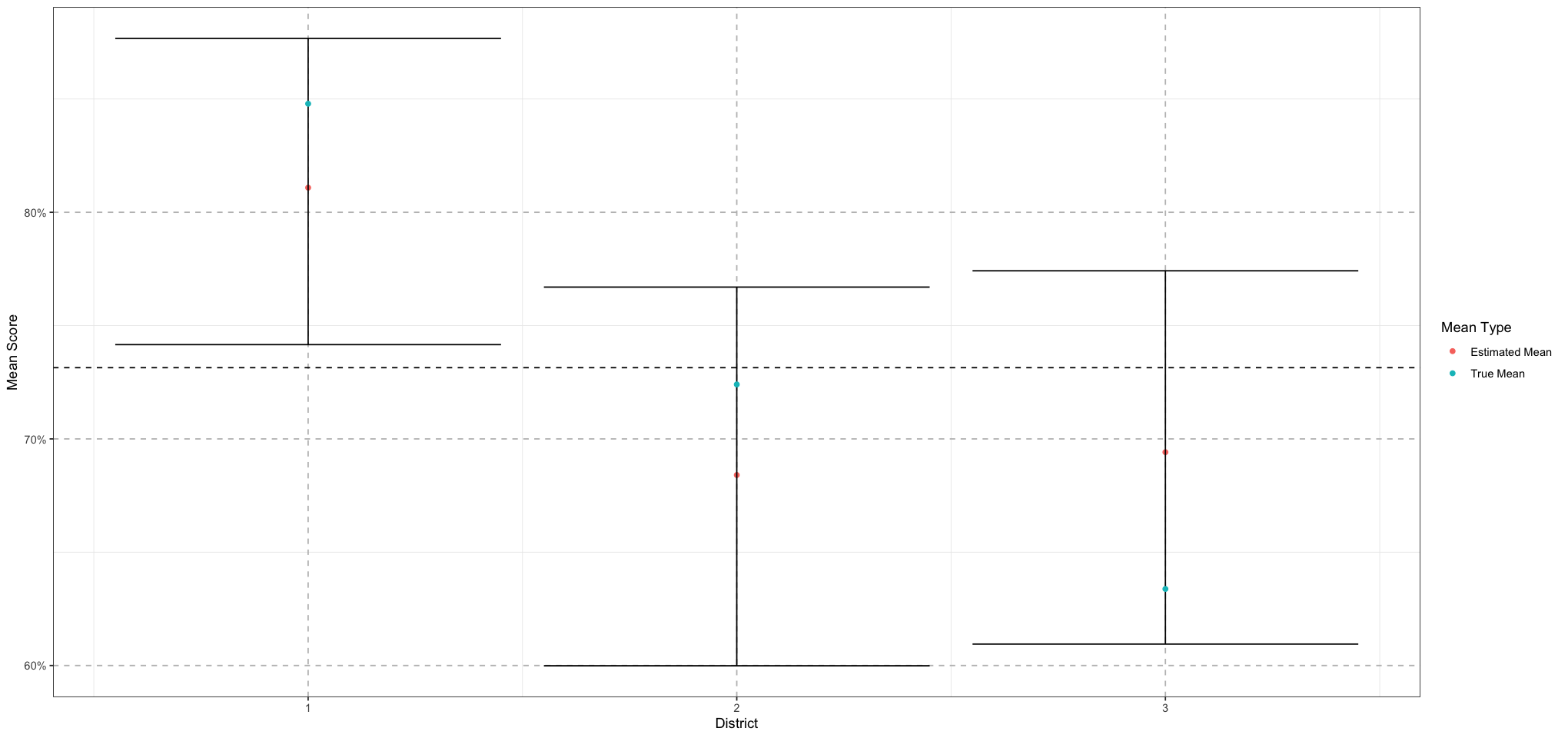
student_school_district_draws <- as_draws_matrix(student_school_district_fit)# Extract district means
district_means_draws <- student_school_district_draws[, grep('mu_district', colnames(student_school_district_draws))]
# Calculate the mean, lower, and upper quantiles for each district
district_mean_means <- apply(district_means_draws, 2, mean)
district_mean_lower <- apply(district_means_draws, 2, function(col) quantile(col, 0.025))
district_mean_upper <- apply(district_means_draws, 2, function(col) quantile(col, 0.975))
# Calculate the mean for the districts
prior_district_mean <- mean(student_school_district_draws[, 'alpha_bar'] / (student_school_district_draws[, 'alpha_bar'] + student_school_district_draws[, 'beta_bar']))
# Create a data frame to store the results
district_means_df <- data.frame(
district = 1:NUM_DISTRICTS,
mean = district_mean_means,
lower = district_mean_lower,
upper = district_mean_upper
)
# Plot the district means along with the true means
ggplot(district_means_df, aes(district, mean)) +
geom_point(aes(colour = "Estimated Mean")) +
geom_errorbar(aes(ymin = lower, ymax = upper)) +
geom_point(data = data.frame(district = 1:NUM_DISTRICTS, mean = district_means), aes(district, mean, colour = "True Mean")) +
geom_hline(yintercept = prior_district_mean, linetype = 'dashed') +
labs(x = "District", y = "Mean Score", colour = "Mean Type") +
scale_y_continuous(labels = scales::percent_format(accuracy = 1)) +
theme_bw() +
theme(
panel.grid.major = element_line(size = 0.5, linetype = 'dashed', colour = "grey"),
)
# Extract school means
school_means_draws <- student_school_district_draws[, grep('mu_school', colnames(student_school_district_draws))]

# Calculate the mean, lower, and upper quantiles for each school
school_mean_means <- apply(school_means_draws, 2, mean)
school_mean_lower <- apply(school_means_draws, 2, function(col) quantile(col, 0.025))
school_mean_upper <- apply(school_means_draws, 2, function(col) quantile(col, 0.975))

district_mean_draws <- student_school_district_draws[, grep('mu_district', colnames(student_school_district_draws))]
district_mean_means <- apply(district_means_draws, 2, mean)

# Create a data frame to store the results
school_means_df <- data.frame(
    school = as.factor(1:TOTAL_SCHOOLS),
    mean = school_mean_means,
    lower = school_mean_lower,
    upper = school_mean_upper
)

# Plot the school means along with the true means
plot <- ggplot(school_means_df, aes(school, mean)) +
    geom_point(aes(colour = "Estimated Mean")) +
    geom_errorbar(aes(ymin = lower, ymax = upper)) +
    geom_point(data = data.frame(school = 1:TOTAL_SCHOOLS, mean = school_params$school_mu), aes(school, mean, colour = "True Mean")) +
    labs(x = "School", y = "Mean Score", colour = "Mean Type") +
    scale_y_continuous(labels = scales::percent_format(accuracy = 1)) +
    theme_bw() +
    theme(
        panel.grid.major = element_line(size = 0.5, linetype = 'dashed', colour = "grey"),
    )

for (district in 1:NUM_DISTRICTS) {
    print(district)
    plot <- plot +
        geom_segment(x = (district - 1) * SCHOOLS_PER_DISTRICT + 0.5, xend = district * SCHOOLS_PER_DISTRICT + 0.5, y = district_mean_means[district], yend = district_mean_means[district], linetype = "dashed")
}

print(plot)
[1] 1
[1] 2
[1] 3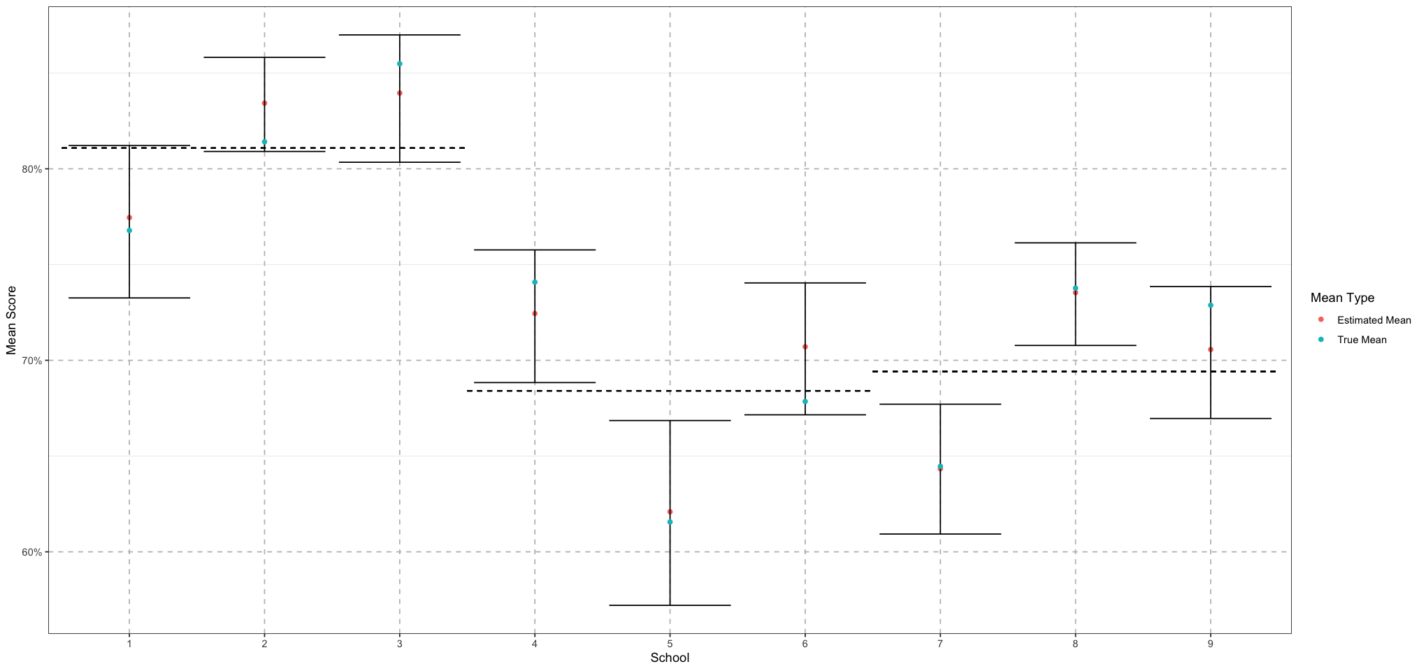
Great! So that worked out pretty well - we’re getting good estimates for both our district-level and school-level values.
So now that we’ve taken a look at a couple of simulated examples, let’s look at some real data: provincial achievement test scores for Alberta!
Example - Alberta Diploma Exam Scores, 2016
Each year, students in Grade 12 in Alberta write diploma exams. These are standardized exams designed to assess the students’ knowledge of different courses. Not every course has a diploma exam, but for those that do, it counts for 30% of their final grade.
Luckily for us, the results of the diploma exam are released publicly, broken up by school, school authority, year, and subject! We’re going to apply the same idea as above to some real data.
The first thing that we need to do is to load in the data. It can be found publicly at the Canada Open Government site. For this, we’ll be looking at the data for the 2015 / 2016 school year.
school_df <- read_excel('data/diploma-multiyear-sch-list-annual.xlsx')
colnames(school_df)- 'Diploma Course'
- 'Authority Type'
- 'Authority Code'
- 'Authority Name'
- 'School Code'
- 'School Name'
- '2012SchStudents Writing'
- '2012Sch School Mark % Exc'
- '2012Sch School Mark % Acc'
- '2012Sch School Average %'
- '2012Sch School Standard Deviation %'
- '2012Sch Exam Mark % Exc'
- '2012Sch Exam Mark Exc Sig'
- '2012Sch Exam Mark % Acc'
- '2012Sch Exam Mark Acc Sig'
- '2012Sch Exam Average %'
- '2012Sch Exam Standard Deviation %'
- '2013Sch Students Writing'
- '2013Sch School Mark % Exc'
- '2013Sch School Mark % Acc'
- '2013Sch School Average %'
- '2013Sch School Standard Deviation %'
- '2013Sch Exam Mark % Exc'
- '2013Sch Exam Mark Exc Sig'
- '2013Sch Exam Mark % Acc'
- '2013Sch Exam Mark Acc Sig'
- '2013Sch Exam Average %'
- '2013Sch Exam Standard Deviation %'
- '2014Sch Students Writing'
- '2014Sch School Mark % Exc'
- '2014Sch School Mark % Acc'
- '2014Sch School Average %'
- '2014Sch School Standard Deviation %'
- '2014Sch Exam Mark % Exc'
- '2014Sch Exam Mark Exc Sig'
- '2014Sch Exam Mark % Acc'
- '2014Sch Exam Mark Acc Sig'
- '2014Sch Exam Average %'
- '2014Sch Exam Standard Deviation %'
- '2015Sch Students Writing'
- '2015Sch School Mark % Exc'
- '2015Sch School Mark % Acc'
- '2015Sch School Average %'
- '2015Sch School Standard Deviation %'
- '2015Sch Exam Mark % Exc'
- '2015Sch Exam Mark Exc Sig'
- '2015Sch Exam Mark % Acc'
- '2015Sch Exam Mark Acc Sig'
- '2015Sch Exam Average %'
- '2015Sch Exam Standard Deviation %'
- '2016Sch Students Writing'
- '2016Sch School Mark % Exc'
- '2016Sch School Mark % Acc'
- '2016Sch School Average %'
- '2016Sch School Standard Deviation %'
- '2016Sch Exam Mark % Exc'
- '2016Sch Exam Mark Exc Sig'
- '2016Sch Exam Mark % Acc'
- '2016Sch Exam Mark Acc Sig'
- '2016Sch Exam Average %'
- '2016Sch Exam Standard Deviation %'
unique(school_df$`Diploma Course`)- 'Biology 30'
- 'Chemistry 30'
- 'English Lang Arts 30-1'
- 'English Lang Arts 30-2'
- 'Mathematics 30-1'
- 'Mathematics 30-2'
- 'Physics 30'
- 'Science 30'
- 'Social Studies 30-1'
- 'Social Studies 30-2'
- 'French Lang Arts 30-1'
- 'Français 30-1'
- '1. The 2012/2013 results do not include students who were exempted from writing the examination because of the flooding in Calgary and southern Alberta.2. The 2015/2016 results do not include students who were exempted from writing the exam because of the Fort McMurray wildfires.3. +,=,- The percentage of students meeting the standard is significantly above (+), not significantly different from (=), or significantly below (-) the previous three-year average. A difference is reported as significant when there is a 5% or smaller probability that a difference of that size could occur by chance. The fewer the number of students, the larger the difference must be from the expectation before it is considered significant. Significance is not calculated for fewer than 6 students.'
Unsuprisingly, there’s a lot here! Let’s focus in - specifically, let’s only look at the Mathematics 30-1 course in 2016. I first taught that course in 2017, so the results here are of some personal interest to me.
relevant_schools_df <- school_df[school_df$`Diploma Course` == 'Mathematics 30-1', c("Diploma Course", "Authority Type", "Authority Code", "Authority Name", "School Code", "School Name", "2016Sch Students Writing", "2016Sch Exam Average %", "2016Sch Exam Standard Deviation %")]

# remove any where no students wrote
relevant_schools_df <- relevant_schools_df[relevant_schools_df$`2016Sch Students Writing` != 'n/a', ]

# convert to numeric
relevant_schools_df$`2016Sch Students Writing` <- as.integer(relevant_schools_df$`2016Sch Students Writing`)
relevant_schools_df$`2016Sch Exam Average %` <- as.numeric(relevant_schools_df$`2016Sch Exam Average %`)
relevant_schools_df$`2016Sch Exam Standard Deviation %` <- as.numeric(relevant_schools_df$`2016Sch Exam Standard Deviation %`)

# codes should be factors
relevant_schools_df$`Authority Code` <- as.factor(relevant_schools_df$`Authority Code`)
relevant_schools_df$`School Code` <- as.factor(relevant_schools_df$`School Code`)

head(relevant_schools_df)| Diploma Course | Authority Type | Authority Code | Authority Name | School Code | School Name | 2016Sch Students Writing | 2016Sch Exam Average % | 2016Sch Exam Standard Deviation % |
|---|---|---|---|---|---|---|---|---|
| <chr> | <chr> | <fct> | <chr> | <fct> | <chr> | <int> | <dbl> | <dbl> |
| Mathematics 30-1 | Charter | 0009 | Foundations for the Future Charter Academy Charter School Society | 0012 | FFCA High School Campus | 113 | 63.9 | 20.0 |
| Mathematics 30-1 | Private | 0015 | Webber Academy Foundation | 0021 | Webber Academy | 59 | 84.8 | 10.8 |
| Mathematics 30-1 | Separate | 0019 | Red Deer Catholic Regional Division No. 39 | 1272 | St. Dominic High School | 12 | 63.3 | 15.5 |
| Mathematics 30-1 | Separate | 0019 | Red Deer Catholic Regional Division No. 39 | 4471 | Ecole Secondaire Notre Dame High School | 190 | 61.8 | 20.0 |
| Mathematics 30-1 | Separate | 0019 | Red Deer Catholic Regional Division No. 39 | 4483 | St. Gabriel Cyber School | 26 | 38.9 | 23.0 |
| Mathematics 30-1 | Separate | 0020 | St. Thomas Aquinas Roman Catholic Separate Regional Division No. 38 | 1328 | Holy Trinity Academy | 10 | 49.0 | 22.4 |
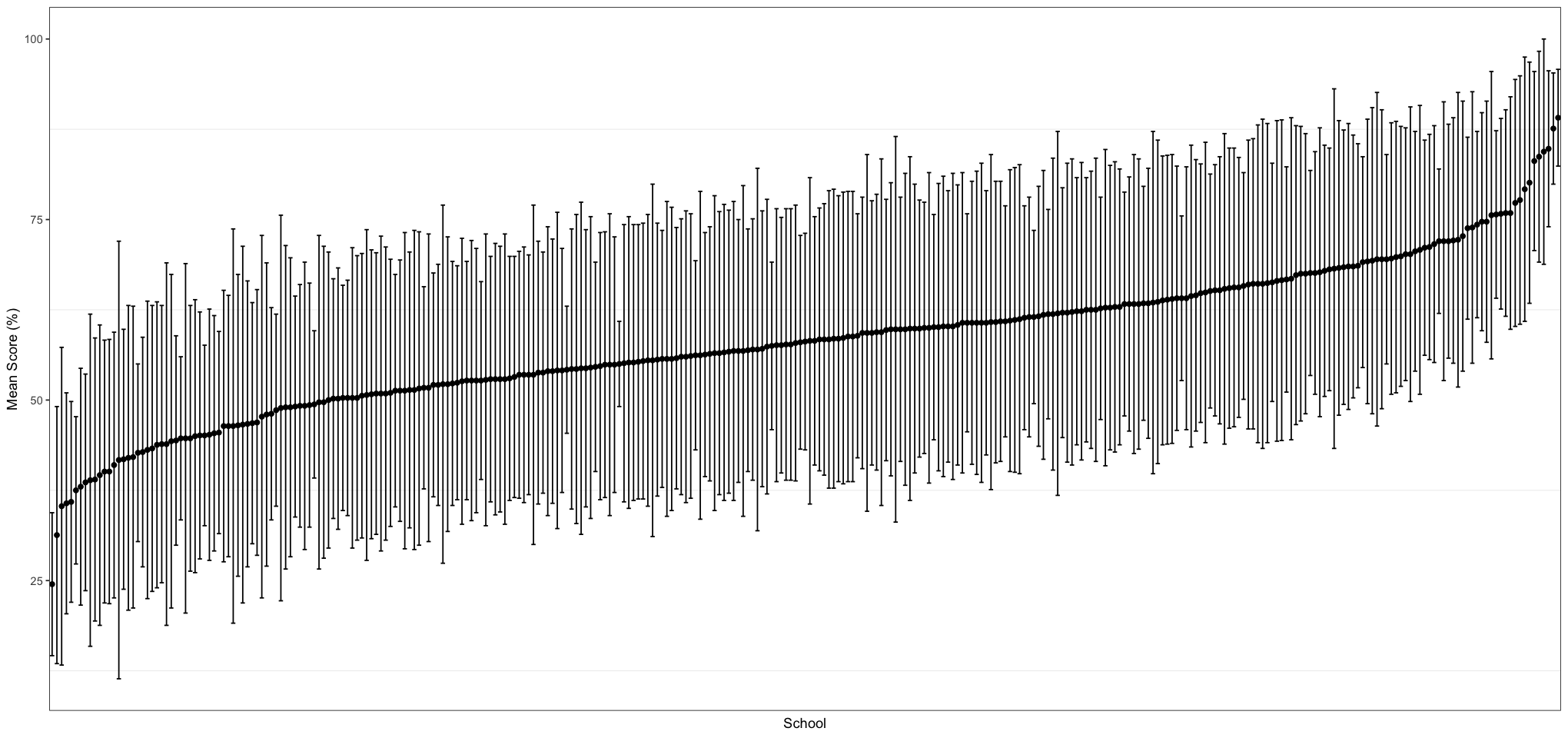
Let’s graph the school results to get a feel for what the data look like:
plot_df <- data.frame(
    school = relevant_schools_df$`School Code`,
    authority = relevant_schools_df$`Authority Code`,
    mean = relevant_schools_df$`2016Sch Exam Average %`,
    lower = relevant_schools_df$`2016Sch Exam Average %` - relevant_schools_df$`2016Sch Exam Standard Deviation %`,
    upper = relevant_schools_df$`2016Sch Exam Average %` + relevant_schools_df$`2016Sch Exam Standard Deviation %`
)
# sort by mean, ascending
plot_df <- plot_df[order(plot_df$mean), ]

# should be plotted in the order of the mean
plot_df$school <- factor(plot_df$school, levels = plot_df$school)

ggplot(plot_df, aes(school, mean)) +
    geom_point() +
    geom_errorbar(aes(ymin = lower, ymax = upper)) +
    labs(x = "School", y = "Mean Score (%)") +
    theme_bw() +
    theme(
        panel.grid.major = element_blank(),
        axis.text.x = element_blank(), axis.ticks.x = element_blank()
    )
There’s definitely an interesting shape to the data! I am a bit shocked by the number of schools with extremely low averages, but such is life I suppose. Let’s see if colouring by the school authority reveals anything.
ggplot(plot_df, aes(school, mean, colour = authority)) +
    geom_point() +
    geom_errorbar(aes(ymin = lower, ymax = upper)) +
    labs(x = "School", y = "Mean Score", colour = "Authority") +
    theme_bw() +
    theme(
        panel.grid.major = element_blank(),
        axis.text.x = element_blank(), axis.ticks.x = element_blank()
    )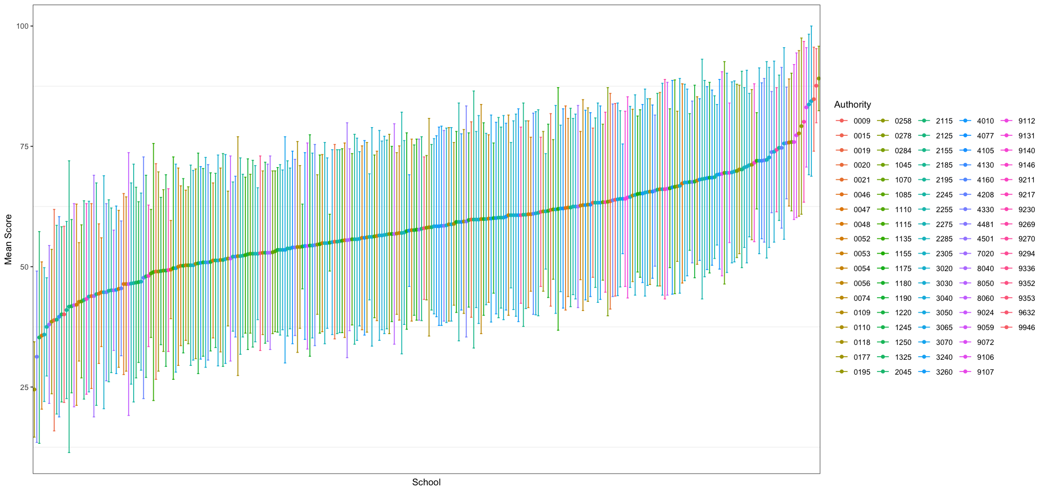
This is some glorious nonsense! Let’s try creating a crude average for the different authorities and plotting that.
authorities_df <- data.frame(authority = unique(relevant_schools_df$`Authority Code`))
authority_means <- sapply(authorities_df$authority, function(authority) {
    authority_schools <- relevant_schools_df[relevant_schools_df$`Authority Code` == authority, ]
    authority_mean <- sum(authority_schools$`2016Sch Exam Average %` * authority_schools$`2016Sch Students Writing`) / sum(authority_schools$`2016Sch Students Writing`)
    authority_mean
})
authority_num_schools <- sapply(authorities_df$authority, function(authority) {
    nrow(relevant_schools_df[relevant_schools_df$`Authority Code` == authority, ])
})

authorities_df$mean <- authority_means
authorities_df$num_schools <- authority_num_schools
# # plot these, ascending
authorities_df <- authorities_df[order(authorities_df$mean), ]
authorities_df$authority <- factor(authorities_df$authority, levels = authorities_df$authority)
ggplot(authorities_df, aes(authority, mean)) +
    geom_point(aes(size = num_schools)) +
    labs(x = "Authority", y = "Mean Score") +
    theme(axis.text.x = element_blank(), axis.ticks.x = element_blank()) +
    theme_bw() +  # Set background to white
    theme(
        panel.grid.major.x = element_blank(),
        panel.grid.minor.x = element_blank(),
        panel.grid.major.y = element_line(size = 0.5, linetype = 'dashed', colour = "grey"),
        axis.ticks.x = element_blank(),
        axis.text.x = element_blank(),
    )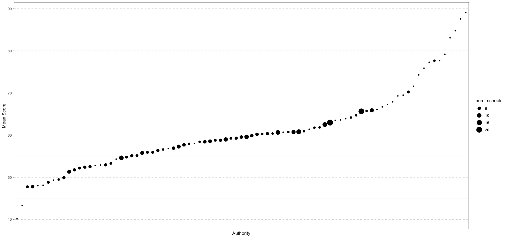
So this looks roughly the same as the earlier graph of the per-school average, except now we’re plotting the per-authority average.
Great! So now let’s try to create a hierarchical model for the results based on the school and the school based on the authority. There is one wrinkle here, which is that for the data that we have, we don’t get the individual student data (unfortunately), which is different from what we’ve considered before. Instead, we’re going to have to create a likelihood from the data which we do have, which is the final mean, standard deviation, and number of students for each school. We’ll also remove any schools where fewer than 30 students wrote the exam.
So here’s our new approach:
- Filter out all of the schools where less than 30 students wrote the exam
- Recalculate the relevant schools and authorities
- Model the likelihood for the sample mean as
Great! So now let’s filter the data.
MIN_STUDENTS <- 30
filtered_schools_df <- relevant_schools_df[relevant_schools_df['2016Sch Students Writing'] >= MIN_STUDENTS, ]
print(paste('Original number of schools:', nrow(relevant_schools_df), 'Filtered number of schools:', nrow(filtered_schools_df)))
[1] "Original number of schools: 317 Filtered number of schools: 140"# plot the schools, ascending
plot_df <- data.frame(
school = filtered_schools_df$`School Code`,
authority = filtered_schools_df$`Authority Code`,
students = filtered_schools_df$`2016Sch Students Writing`,
mean = filtered_schools_df$`2016Sch Exam Average %`,
lower = filtered_schools_df$`2016Sch Exam Average %` - filtered_schools_df$`2016Sch Exam Standard Deviation %`,
upper = filtered_schools_df$`2016Sch Exam Average %` + filtered_schools_df$`2016Sch Exam Standard Deviation %`
)
# sort by mean, ascending
plot_df <- plot_df[order(plot_df$mean), ]
# should be plotted in the order of the mean
plot_df$school <- factor(plot_df$school, levels = plot_df$school)
ggplot(plot_df, aes(school, mean)) +
geom_point(aes(size = students)) +
geom_errorbar(aes(ymin = lower, ymax = upper)) +
labs(x = "School", y = "Mean Score") +
theme_bw() +
theme(
panel.grid.major.x = element_blank(),
panel.grid.minor.x = element_blank(),
panel.grid.major.y = element_line(size = 0.5, linetype = 'dashed', colour = "grey"),
axis.ticks.x = element_blank(),
axis.text.x = element_blank(),
)
# now handle the authorities
authorities_df <- data.frame(authority = unique(filtered_schools_df$`Authority Code`))
authority_means <- sapply(authorities_df$authority, function(authority) {
authority_schools <- filtered_schools_df[filtered_schools_df$`Authority Code` == authority, ]
authority_mean <- sum(authority_schools$`2016Sch Exam Average %` * authority_schools$`2016Sch Students Writing`) / sum(authority_schools$`2016Sch Students Writing`)
authority_mean
})
authority_num_schools <- sapply(authorities_df$authority, function(authority) {
nrow(filtered_schools_df[filtered_schools_df$`Authority Code` == authority, ])
})
authorities_df$mean <- authority_means
authorities_df$num_schools <- authority_num_schools
# # plot the authorities, ascending
authorities_df <- authorities_df[order(authorities_df$mean), ]
authorities_df$authority <- factor(authorities_df$authority, levels = authorities_df$authority)
ggplot(authorities_df, aes(authority, mean)) +
geom_point(aes(size = num_schools)) +
labs(x = "Authority", y = "Mean Score", size = "Number of Schools") +
theme_bw() +
theme(
panel.grid.major.x = element_blank(),
panel.grid.minor.x = element_blank(),
panel.grid.major.y = element_line(size = 0.5, linetype = 'dashed', colour = "grey"),
axis.ticks.x = element_blank(),
axis.text.x = element_blank(),
)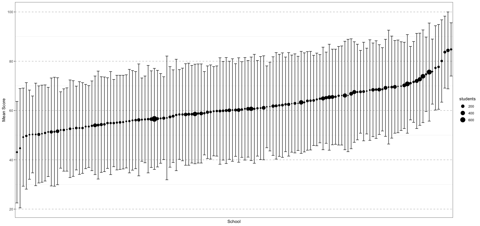
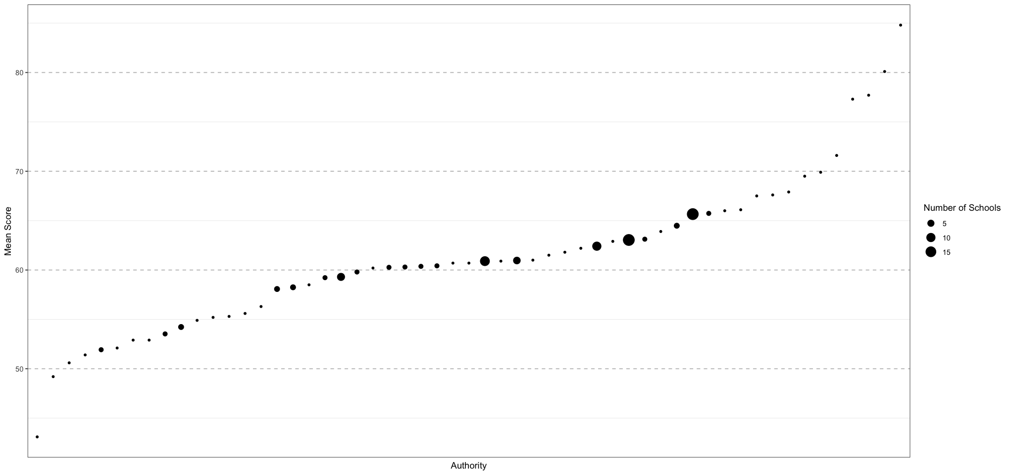
By looking at the graphs, we see that the underlying shape hasn’t changed too much by removing the schools with fewer students; we’ve just trimmed it down a bit. Now let’s build the model! As before, we’ll start with the unpooled model, then pool all of the schools together, then finally pooly by district.
# convert the authorities to indices
authority_df <- data.frame(
    authority = unique(filtered_schools_df$`Authority Code`),
    index = seq_along(1:length(unique(filtered_schools_df$`Authority Code`)))
)
authority_index <- authority_df$index[match(filtered_schools_df$`Authority Code`, authority_df$authority)]
alberta_schools_data <- list(
    N_schools = nrow(filtered_schools_df),
    N_authorities = length(unique(filtered_schools_df$`Authority Code`)),
    authority_index = authority_index,
    school_mean = filtered_schools_df$`2016Sch Exam Average %` / 100,
    school_s_squared = (filtered_schools_df$`2016Sch Exam Standard Deviation %` / 100)^2,
    school_n = filtered_schools_df$`2016Sch Students Writing`
)

run_schools_model <- function(model_code_string) {
    model_file <- write_stan_file(model_code_string)
    model <- cmdstan_model(model_file)
    model_fit <- model$sample(
        data = alberta_schools_data,
        chains = 4,
        iter_warmup = 1000,
        adapt_delta = 0.99
    )
    model_fit
}

alberta_schools_unpooled_code <- "
data {
    int<lower = 0> N_schools;
    array[N_schools] real<lower = 0, upper = 1> school_mean;
    array[N_schools] int<lower = 0> school_n;
}
parameters {
    array[N_schools] real<lower = 0, upper = 1> school_mu;
    array[N_schools] real<lower = 0> school_nu;
}
transformed parameters {
    array[N_schools] real<lower = 0> school_alpha;
    array[N_schools] real<lower = 0> school_beta;
    array[N_schools] real<lower = 0> school_sigma_squared;
    for (i in 1:N_schools) {
        school_alpha[i] = school_mu[i] * school_nu[i];
        school_beta[i] = (1 - school_mu[i]) * school_nu[i];
        school_sigma_squared[i] = (school_alpha[i] * school_beta[i]) / (( school_alpha[i] + school_beta[i])^2 * (school_alpha[i] + school_beta[i] + 1));
    }
}
model {
    for (i in 1:N_schools) {
        school_mean[i] ~ normal(school_mu[i], sqrt(school_sigma_squared[i] / school_n[i]));
    }
    school_mu ~ beta(3, 1);
    school_nu ~ normal(30, 4);
}
"

alberta_schools_unpooled_fit <- run_schools_model(alberta_schools_unpooled_code)
alberta_schools_unpooled_fit$summary()
Running MCMC with 4 sequential chains...
All 4 chains finished successfully.
Mean chain execution time: 3.5 seconds.
Total execution time: 14.4 seconds.| variable | mean | median | sd | mad | q5 | q95 | rhat | ess_bulk | ess_tail |
|---|---|---|---|---|---|---|---|---|---|
| <chr> | <dbl> | <dbl> | <dbl> | <dbl> | <dbl> | <dbl> | <dbl> | <dbl> | <dbl> |
| lp__ | 649.5773287 | 649.7755000 | 12.201033065 | 12.312993000 | 629.2904000 | 669.0576000 | 1.0029001 | 1430.923 | 2053.862 |
| school_mu[1] | 0.6392039 | 0.6393735 | 0.008405132 | 0.008324058 | 0.6248339 | 0.6527770 | 1.0023608 | 9861.831 | 3085.230 |
| school_mu[2] | 0.8478341 | 0.8478955 | 0.008545827 | 0.008547189 | 0.8338857 | 0.8613602 | 1.0026531 | 10923.645 | 2489.053 |
| school_mu[3] | 0.6181320 | 0.6181990 | 0.006292014 | 0.006273622 | 0.6079128 | 0.6282794 | 1.0005929 | 9275.417 | 2710.679 |
| school_mu[4] | 0.6221342 | 0.6222265 | 0.008266059 | 0.008361123 | 0.6085825 | 0.6353736 | 1.0003571 | 8557.712 | 2885.691 |
| school_mu[5] | 0.6091299 | 0.6094770 | 0.010714624 | 0.010414524 | 0.5915248 | 0.6270132 | 1.0001241 | 9395.256 | 2746.722 |
| school_mu[6] | 0.5643965 | 0.5645085 | 0.012238623 | 0.012046125 | 0.5443312 | 0.5843314 | 1.0013317 | 10665.311 | 2956.641 |
| school_mu[7] | 0.7579158 | 0.7584285 | 0.013581550 | 0.013060965 | 0.7342792 | 0.7798935 | 1.0003750 | 11019.426 | 2544.310 |
| school_mu[8] | 0.6613427 | 0.6616730 | 0.015752203 | 0.015415333 | 0.6350851 | 0.6866007 | 1.0003204 | 9957.812 | 3062.898 |
| school_mu[9] | 0.5039022 | 0.5035950 | 0.015266937 | 0.015177376 | 0.4785290 | 0.5287871 | 1.0001035 | 9218.511 | 2836.723 |
| school_mu[10] | 0.5495140 | 0.5494805 | 0.010088190 | 0.010011998 | 0.5330208 | 0.5663486 | 1.0020066 | 9635.417 | 2255.971 |
| school_mu[11] | 0.6074124 | 0.6077090 | 0.013410985 | 0.013212931 | 0.5844894 | 0.6287470 | 1.0013039 | 10233.535 | 2432.842 |
| school_mu[12] | 0.6794369 | 0.6794635 | 0.014992119 | 0.014513913 | 0.6545396 | 0.7037216 | 1.0017366 | 9346.925 | 2523.928 |
| school_mu[13] | 0.7769397 | 0.7770205 | 0.008391946 | 0.008506418 | 0.7629991 | 0.7904530 | 1.0006798 | 10609.349 | 3094.103 |
| school_mu[14] | 0.5941705 | 0.5941310 | 0.009878963 | 0.009741423 | 0.5780519 | 0.6106447 | 0.9999009 | 9063.377 | 2557.421 |
| school_mu[15] | 0.5822358 | 0.5823065 | 0.010688901 | 0.010906747 | 0.5647210 | 0.5995771 | 0.9998798 | 8514.371 | 2849.397 |
| school_mu[16] | 0.5612107 | 0.5611500 | 0.009223588 | 0.008926735 | 0.5459749 | 0.5764008 | 1.0015537 | 9275.307 | 2389.068 |
| school_mu[17] | 0.6562535 | 0.6564125 | 0.009768611 | 0.009671000 | 0.6395904 | 0.6720952 | 1.0010295 | 8951.184 | 2822.084 |
| school_mu[18] | 0.7020372 | 0.7021400 | 0.005097796 | 0.005126831 | 0.6936178 | 0.7103156 | 1.0021930 | 8503.081 | 3030.269 |
| school_mu[19] | 0.5692039 | 0.5691785 | 0.007228040 | 0.007006026 | 0.5572946 | 0.5811564 | 1.0009770 | 9479.563 | 2602.059 |
| school_mu[20] | 0.6291591 | 0.6291845 | 0.007741292 | 0.007446359 | 0.6163890 | 0.6421733 | 1.0009216 | 9699.631 | 2890.812 |
| school_mu[21] | 0.5291810 | 0.5291255 | 0.009326573 | 0.009361878 | 0.5138633 | 0.5444111 | 1.0025134 | 9776.379 | 2905.082 |
| school_mu[22] | 0.6482721 | 0.6483485 | 0.010462342 | 0.010331498 | 0.6312333 | 0.6653092 | 1.0003151 | 8538.696 | 2790.360 |
| school_mu[23] | 0.5894198 | 0.5894010 | 0.010529789 | 0.010301846 | 0.5720068 | 0.6064943 | 1.0013085 | 9797.334 | 2746.159 |
| school_mu[24] | 0.5411187 | 0.5410025 | 0.007940582 | 0.007633166 | 0.5281375 | 0.5540133 | 1.0017240 | 11054.748 | 2125.300 |
| school_mu[25] | 0.5883560 | 0.5882275 | 0.010369037 | 0.010146173 | 0.5711747 | 0.6053831 | 1.0002894 | 9185.769 | 2727.709 |
| school_mu[26] | 0.5070336 | 0.5072020 | 0.015308408 | 0.014958693 | 0.4821989 | 0.5320383 | 1.0011184 | 9601.298 | 2389.797 |
| school_mu[27] | 0.6153622 | 0.6153640 | 0.015527387 | 0.015326377 | 0.5900032 | 0.6408760 | 1.0014148 | 9793.679 | 2783.556 |
| school_mu[28] | 0.6994129 | 0.6996925 | 0.014865654 | 0.014537634 | 0.6749133 | 0.7232319 | 1.0053603 | 9952.072 | 2730.345 |
| school_mu[29] | 0.6951703 | 0.6954805 | 0.014038333 | 0.014172915 | 0.6723685 | 0.7179155 | 1.0009009 | 9118.153 | 2701.306 |
| ⋮ | ⋮ | ⋮ | ⋮ | ⋮ | ⋮ | ⋮ | ⋮ | ⋮ | ⋮ |
| school_sigma_squared[111] | 0.007893264 | 0.007768190 | 0.0010697738 | 0.0010081383 | 0.006439076 | 0.009800432 | 1.0004525 | 7428.400 | 2527.758 |
| school_sigma_squared[112] | 0.007969189 | 0.007832225 | 0.0010926129 | 0.0010291023 | 0.006428079 | 0.009930932 | 1.0020825 | 10505.973 | 2602.756 |
| school_sigma_squared[113] | 0.007618596 | 0.007507175 | 0.0010481282 | 0.0010130680 | 0.006157625 | 0.009520502 | 1.0014516 | 8158.273 | 2472.058 |
| school_sigma_squared[114] | 0.007964497 | 0.007842500 | 0.0010674834 | 0.0010013036 | 0.006464247 | 0.009853104 | 1.0000604 | 8319.391 | 2477.557 |
| school_sigma_squared[115] | 0.007830389 | 0.007684080 | 0.0010859503 | 0.0010140984 | 0.006311180 | 0.009815478 | 1.0037708 | 8275.381 | 2041.495 |
| school_sigma_squared[116] | 0.007643599 | 0.007525235 | 0.0010180235 | 0.0009446608 | 0.006205853 | 0.009519544 | 1.0012818 | 9034.527 | 3076.640 |
| school_sigma_squared[117] | 0.007079024 | 0.006956720 | 0.0009694878 | 0.0008953644 | 0.005748352 | 0.008871571 | 1.0016213 | 9660.773 | 2506.069 |
| school_sigma_squared[118] | 0.007978155 | 0.007838450 | 0.0010765993 | 0.0010081087 | 0.006465149 | 0.009911454 | 1.0020249 | 8893.435 | 2733.333 |
| school_sigma_squared[119] | 0.007435998 | 0.007330955 | 0.0009979564 | 0.0009291677 | 0.005993480 | 0.009225692 | 1.0004015 | 8705.208 | 2244.065 |
| school_sigma_squared[120] | 0.007003157 | 0.006878335 | 0.0009683727 | 0.0008945860 | 0.005693553 | 0.008771605 | 1.0006612 | 10321.591 | 2666.727 |
| school_sigma_squared[121] | 0.007845839 | 0.007733620 | 0.0010310463 | 0.0009563511 | 0.006429796 | 0.009630830 | 1.0029224 | 9922.761 | 2363.052 |
| school_sigma_squared[122] | 0.007879970 | 0.007717540 | 0.0011086189 | 0.0009984718 | 0.006355423 | 0.009884213 | 1.0027917 | 9441.005 | 2877.827 |
| school_sigma_squared[123] | 0.007090519 | 0.006984445 | 0.0009657778 | 0.0009240230 | 0.005747343 | 0.008932001 | 1.0010618 | 10143.593 | 2668.185 |
| school_sigma_squared[124] | 0.008151195 | 0.008004090 | 0.0011242317 | 0.0010409186 | 0.006603203 | 0.010195930 | 0.9999701 | 9655.258 | 2639.273 |
| school_sigma_squared[125] | 0.008142819 | 0.008005325 | 0.0010949668 | 0.0010205032 | 0.006658687 | 0.010109410 | 1.0020682 | 10818.940 | 2288.183 |
| school_sigma_squared[126] | 0.007719722 | 0.007619380 | 0.0010202034 | 0.0009789830 | 0.006292084 | 0.009589083 | 1.0026693 | 7682.836 | 2778.122 |
| school_sigma_squared[127] | 0.008047316 | 0.007917465 | 0.0010627631 | 0.0010092132 | 0.006559594 | 0.009984389 | 1.0030703 | 10158.718 | 2560.377 |
| school_sigma_squared[128] | 0.007639193 | 0.007519170 | 0.0010104833 | 0.0009244826 | 0.006201755 | 0.009444058 | 1.0009677 | 9342.876 | 2821.260 |
| school_sigma_squared[129] | 0.008200299 | 0.008042745 | 0.0011332436 | 0.0010339059 | 0.006623680 | 0.010261805 | 0.9997888 | 9525.584 | 2875.477 |
| school_sigma_squared[130] | 0.007805796 | 0.007658680 | 0.0010914395 | 0.0009610139 | 0.006333933 | 0.009777402 | 1.0011799 | 6632.328 | 2140.112 |
| school_sigma_squared[131] | 0.007209483 | 0.007093005 | 0.0010073930 | 0.0009162839 | 0.005841421 | 0.009100803 | 1.0009968 | 8307.831 | 2324.168 |
| school_sigma_squared[132] | 0.007963293 | 0.007820475 | 0.0010980682 | 0.0009929862 | 0.006425254 | 0.009945242 | 1.0013978 | 9306.196 | 2473.790 |
| school_sigma_squared[133] | 0.008199732 | 0.008062010 | 0.0011416851 | 0.0010541953 | 0.006616617 | 0.010259080 | 1.0001760 | 8278.864 | 2319.211 |
| school_sigma_squared[134] | 0.007685228 | 0.007556640 | 0.0010438796 | 0.0009747502 | 0.006244291 | 0.009554043 | 1.0022049 | 7625.178 | 2862.585 |
| school_sigma_squared[135] | 0.007994192 | 0.007853765 | 0.0010924612 | 0.0010112296 | 0.006505752 | 0.010028570 | 1.0015995 | 7389.714 | 2102.009 |
| school_sigma_squared[136] | 0.008093561 | 0.007955880 | 0.0011403109 | 0.0010455888 | 0.006541122 | 0.010090635 | 1.0010682 | 9287.799 | 2156.026 |
| school_sigma_squared[137] | 0.005750439 | 0.005664375 | 0.0007842457 | 0.0007583647 | 0.004663566 | 0.007139022 | 0.9996415 | 9412.067 | 2355.305 |
| school_sigma_squared[138] | 0.006652218 | 0.006531960 | 0.0008836756 | 0.0008276392 | 0.005436707 | 0.008254424 | 1.0006992 | 8224.799 | 2692.735 |
| school_sigma_squared[139] | 0.005245804 | 0.005143150 | 0.0007534517 | 0.0007090460 | 0.004210688 | 0.006630924 | 1.0002898 | 9417.638 | 2560.559 |
| school_sigma_squared[140] | 0.007339370 | 0.007229320 | 0.0009939939 | 0.0009337711 | 0.005963415 | 0.009117067 | 0.9999096 | 9246.506 | 2855.895 |
generate_school_plot <- function(fit) {
    draws <- as_draws_matrix(fit)

    plot_df <- data.frame(
        school = filtered_schools_df$`School Code`,
        students = filtered_schools_df$`2016Sch Students Writing`,
        observed_mean = filtered_schools_df$`2016Sch Exam Average %` / 100,
        observed_lower = filtered_schools_df$`2016Sch Exam Average %` / 100 - filtered_schools_df$`2016Sch Exam Standard Deviation %` / 100,
        observed_upper = filtered_schools_df$`2016Sch Exam Average %` / 100 + filtered_schools_df$`2016Sch Exam Standard Deviation %` / 100,
        model_mean = colMeans(draws[, grep('school_mu', colnames(draws))]),
        model_lower = apply(draws[, grep('school_mu', colnames(draws))], 2, function(col) quantile(col, 0.025)),
        model_upper = apply(draws[, grep('school_mu', colnames(draws))], 2, function(col) quantile(col, 0.975))
    )
    plot_df <- plot_df[order(plot_df$observed_mean), ]
    plot_df$school <- factor(plot_df$school, levels = plot_df$school)
    # plot the empirical data against the estimated means
    p <- ggplot(plot_df) +
        geom_point(aes(school, observed_mean, size = students, colour = "Observed")) +
        geom_point(aes(school, model_mean, colour = 'Model')) +
        geom_errorbar(aes(x = school, y = model_mean, ymin = model_lower, ymax = model_upper, colour = "Model")) +
        labs(x = "School", y = "Mean Score", size = "Number of Students", colour = "") +
        scale_y_continuous(labels = scales::percent_format(accuracy = 1)) +
        theme_bw() +  # Set background to white
        theme(
            panel.grid.major.x = element_blank(),
            panel.grid.minor.x = element_blank(),
            panel.grid.major.y = element_line(size = 0.5, linetype = 'dashed', colour = "grey"),
            axis.ticks.x = element_blank(),
            axis.text.x = element_blank(),
        )
    p
}

unpooled_school_means_plot <- generate_school_plot(alberta_schools_unpooled_fit)
print(unpooled_school_means_plot)
That looks pretty good! Now let’s pool all of the schools together using a shared prior.
alberta_schools_pooled_code <- "
data {
    int<lower = 0> N_schools;
    array[N_schools] real<lower = 0, upper = 1> school_mean;
    array[N_schools] int<lower = 0> school_n;
}
parameters {
    array[N_schools] real<lower = 0, upper = 1> school_mu;
    array[N_schools] real<lower = 0> school_nu_raw; // non-centred - implies school_nu ~ normal(school_prior_nu_mean, school_prior_nu_sd)

    real <lower = 0> school_prior_alpha;
    real <lower = 0> school_prior_beta;
    real <lower = 0> school_prior_nu_mean;
    real <lower = 0> school_prior_nu_sd;
}
transformed parameters {
    array[N_schools] real<lower = 0> school_alpha;
    array[N_schools] real<lower = 0> school_beta;
    array[N_schools] real<lower = 0> school_sigma_squared;
    array[N_schools] real<lower = 0> school_nu;
    for (i in 1:N_schools) {
        school_nu[i] = school_prior_nu_mean + school_prior_nu_sd * school_nu_raw[i];
        school_alpha[i] = school_mu[i] * school_nu[i];
        school_beta[i] = (1 - school_mu[i]) * school_nu[i];
        school_sigma_squared[i] = (school_alpha[i] * school_beta[i]) / (( school_alpha[i] + school_beta[i])^2 * (school_alpha[i] + school_beta[i] + 1));
    }
}
model {
    for (i in 1:N_schools) {
        school_mean[i] ~ normal(school_mu[i], sqrt(school_sigma_squared[i] / school_n[i]));
    }
    school_mu ~ beta(school_prior_alpha, school_prior_beta);
    school_nu_raw ~ std_normal();

    school_prior_alpha ~ normal(3, 0.5);
    school_prior_beta ~ normal(1, 0.3);
    school_prior_nu_mean ~ normal(30, 4);
    school_prior_nu_sd ~ exponential(1);
}
"

alberta_schools_pooled_fit <- run_schools_model(alberta_schools_pooled_code)
alberta_schools_pooled_fit$summary()
Running MCMC with 4 sequential chains...
All 4 chains finished successfully.
Mean chain execution time: 7.3 seconds.
Total execution time: 29.3 seconds.| variable | mean | median | sd | mad | q5 | q95 | rhat | ess_bulk | ess_tail |
|---|---|---|---|---|---|---|---|---|---|
| <chr> | <dbl> | <dbl> | <dbl> | <dbl> | <dbl> | <dbl> | <dbl> | <dbl> | <dbl> |
| lp__ | 303.3768817 | 303.9490000 | 16.010609953 | 15.280416900 | 276.3478500 | 328.5250000 | 1.0015113 | 893.8268 | 1506.195 |
| school_mu[1] | 0.6390792 | 0.6389565 | 0.008087173 | 0.008065344 | 0.6256816 | 0.6524580 | 1.0024593 | 4588.5802 | 3114.740 |
| school_mu[2] | 0.8472796 | 0.8473785 | 0.008252892 | 0.008267719 | 0.8334421 | 0.8606413 | 1.0009509 | 4664.1656 | 2717.473 |
| school_mu[3] | 0.6180220 | 0.6181105 | 0.006271633 | 0.006166133 | 0.6076868 | 0.6283191 | 1.0017390 | 4661.0568 | 3093.812 |
| school_mu[4] | 0.6220444 | 0.6221355 | 0.008126488 | 0.008079429 | 0.6084968 | 0.6352612 | 1.0018828 | 4967.9453 | 3136.635 |
| school_mu[5] | 0.6090356 | 0.6091480 | 0.010636975 | 0.010635431 | 0.5912527 | 0.6262207 | 1.0002508 | 4984.4110 | 2805.612 |
| school_mu[6] | 0.5643344 | 0.5645605 | 0.011741694 | 0.011797048 | 0.5449506 | 0.5838678 | 1.0006932 | 4318.7214 | 2945.927 |
| school_mu[7] | 0.7572024 | 0.7575620 | 0.013173178 | 0.013160299 | 0.7349491 | 0.7783756 | 0.9999079 | 4704.4222 | 2625.790 |
| school_mu[8] | 0.6605515 | 0.6607250 | 0.015465255 | 0.015314517 | 0.6343163 | 0.6858114 | 1.0002815 | 4391.0870 | 2871.989 |
| school_mu[9] | 0.5038833 | 0.5039180 | 0.015056639 | 0.015186272 | 0.4792564 | 0.5281737 | 1.0010799 | 5395.6317 | 2740.259 |
| school_mu[10] | 0.5492591 | 0.5494235 | 0.010111278 | 0.010022376 | 0.5324129 | 0.5659195 | 1.0012927 | 4671.2267 | 2758.982 |
| school_mu[11] | 0.6073463 | 0.6074625 | 0.013313283 | 0.013341917 | 0.5854852 | 0.6290895 | 1.0020000 | 4909.1898 | 2668.409 |
| school_mu[12] | 0.6782184 | 0.6787230 | 0.014706708 | 0.015006136 | 0.6538240 | 0.7014432 | 1.0012839 | 4657.2681 | 2982.858 |
| school_mu[13] | 0.7765780 | 0.7767805 | 0.008369508 | 0.008294406 | 0.7624945 | 0.7903953 | 1.0022197 | 4809.6645 | 2783.120 |
| school_mu[14] | 0.5941792 | 0.5943005 | 0.009515127 | 0.009766628 | 0.5786709 | 0.6097708 | 1.0023599 | 5141.7190 | 2850.491 |
| school_mu[15] | 0.5822526 | 0.5823935 | 0.010862116 | 0.010788880 | 0.5644139 | 0.6000414 | 0.9997710 | 5552.0371 | 3009.097 |
| school_mu[16] | 0.5612144 | 0.5611465 | 0.009131184 | 0.009202498 | 0.5463539 | 0.5758237 | 1.0022781 | 4576.8798 | 2877.150 |
| school_mu[17] | 0.6560447 | 0.6561910 | 0.010477979 | 0.010462708 | 0.6388660 | 0.6728194 | 1.0020644 | 4727.2855 | 2872.770 |
| school_mu[18] | 0.7019719 | 0.7019980 | 0.004950784 | 0.004878495 | 0.6937125 | 0.7101738 | 1.0000035 | 4318.3077 | 3191.356 |
| school_mu[19] | 0.5690055 | 0.5690850 | 0.007141884 | 0.007216556 | 0.5573088 | 0.5803989 | 0.9995899 | 4456.1963 | 3119.883 |
| school_mu[20] | 0.6287745 | 0.6287395 | 0.007553180 | 0.007547175 | 0.6164030 | 0.6412437 | 0.9994805 | 4260.8254 | 3093.037 |
| school_mu[21] | 0.5293484 | 0.5295380 | 0.009045090 | 0.009111318 | 0.5146197 | 0.5441755 | 1.0006101 | 5183.6144 | 3166.340 |
| school_mu[22] | 0.6478409 | 0.6479130 | 0.010385516 | 0.010494584 | 0.6308290 | 0.6643548 | 1.0005523 | 4699.0893 | 3190.544 |
| school_mu[23] | 0.5893679 | 0.5892725 | 0.010550171 | 0.010570197 | 0.5720445 | 0.6067484 | 1.0017835 | 5601.2755 | 3042.860 |
| school_mu[24] | 0.5410172 | 0.5408530 | 0.008148151 | 0.008352227 | 0.5278048 | 0.5544735 | 0.9993166 | 4670.5756 | 2990.563 |
| school_mu[25] | 0.5877308 | 0.5877460 | 0.009933401 | 0.009825932 | 0.5711710 | 0.6040176 | 1.0008139 | 4943.8628 | 2533.125 |
| school_mu[26] | 0.5065683 | 0.5063280 | 0.015377681 | 0.015707406 | 0.4820062 | 0.5320932 | 1.0022437 | 5312.7353 | 2943.792 |
| school_mu[27] | 0.6150520 | 0.6149875 | 0.015574998 | 0.015925348 | 0.5894119 | 0.6402502 | 1.0002420 | 4431.5376 | 2993.436 |
| school_mu[28] | 0.6987703 | 0.6987035 | 0.014475063 | 0.014868254 | 0.6752261 | 0.7222509 | 1.0011157 | 4728.1448 | 2926.576 |
| school_mu[29] | 0.6943627 | 0.6943935 | 0.013998895 | 0.013949783 | 0.6707471 | 0.7169856 | 1.0006656 | 4834.9427 | 2654.505 |
| ⋮ | ⋮ | ⋮ | ⋮ | ⋮ | ⋮ | ⋮ | ⋮ | ⋮ | ⋮ |
| school_nu[111] | 30.78090 | 30.82385 | 4.101406 | 4.041642 | 24.03228 | 37.58628 | 1.0005771 | 1472.580 | 1875.910 |
| school_nu[112] | 30.80212 | 30.71015 | 4.155457 | 4.101242 | 23.99994 | 37.52887 | 1.0003763 | 1475.403 | 1967.981 |
| school_nu[113] | 30.78881 | 30.76595 | 4.128469 | 4.117773 | 24.13262 | 37.50174 | 0.9999277 | 1471.802 | 1808.811 |
| school_nu[114] | 30.80189 | 30.78960 | 4.130428 | 4.069737 | 24.06187 | 37.53622 | 1.0002736 | 1472.135 | 1782.622 |
| school_nu[115] | 30.78738 | 30.75695 | 4.115737 | 4.065586 | 24.05419 | 37.54105 | 1.0001634 | 1463.730 | 1951.738 |
| school_nu[116] | 30.76124 | 30.75665 | 4.130047 | 4.096424 | 24.02190 | 37.54741 | 1.0001140 | 1467.214 | 1807.532 |
| school_nu[117] | 30.78732 | 30.77025 | 4.105511 | 4.035860 | 24.06202 | 37.46641 | 0.9998391 | 1457.559 | 1697.574 |
| school_nu[118] | 30.77963 | 30.77405 | 4.118421 | 4.077076 | 24.03529 | 37.62413 | 1.0000245 | 1453.870 | 1776.225 |
| school_nu[119] | 30.78651 | 30.78055 | 4.138759 | 4.055356 | 24.06464 | 37.46353 | 1.0001119 | 1451.447 | 1861.304 |
| school_nu[120] | 30.80518 | 30.83210 | 4.136719 | 4.043866 | 24.02471 | 37.53602 | 1.0003245 | 1428.196 | 1799.062 |
| school_nu[121] | 30.79084 | 30.74740 | 4.132359 | 4.059729 | 24.09940 | 37.46145 | 1.0002736 | 1447.110 | 1900.183 |
| school_nu[122] | 30.76768 | 30.79925 | 4.095244 | 4.018810 | 24.09209 | 37.46993 | 1.0000350 | 1452.188 | 1818.884 |
| school_nu[123] | 30.79588 | 30.80065 | 4.115233 | 4.056764 | 24.06658 | 37.54259 | 0.9998784 | 1483.732 | 1780.509 |
| school_nu[124] | 30.78983 | 30.80970 | 4.140070 | 4.113325 | 24.04521 | 37.54612 | 1.0003622 | 1448.044 | 1807.375 |
| school_nu[125] | 30.79457 | 30.79990 | 4.119491 | 4.058766 | 24.09196 | 37.57005 | 1.0003071 | 1460.175 | 1883.421 |
| school_nu[126] | 30.78053 | 30.81370 | 4.110078 | 4.089307 | 24.12297 | 37.50183 | 1.0004938 | 1418.450 | 1938.605 |
| school_nu[127] | 30.79112 | 30.80010 | 4.137164 | 4.091902 | 24.13109 | 37.51491 | 1.0001893 | 1456.566 | 1874.482 |
| school_nu[128] | 30.78242 | 30.79370 | 4.099799 | 4.035415 | 24.08486 | 37.60762 | 1.0001670 | 1452.210 | 1833.954 |
| school_nu[129] | 30.77612 | 30.77305 | 4.095918 | 4.020292 | 24.08069 | 37.46192 | 1.0002709 | 1454.949 | 1808.966 |
| school_nu[130] | 30.79206 | 30.78095 | 4.135395 | 4.103392 | 24.04835 | 37.42886 | 0.9998866 | 1433.656 | 1889.972 |
| school_nu[131] | 30.79639 | 30.81580 | 4.106577 | 4.074111 | 24.04705 | 37.46138 | 0.9998806 | 1474.317 | 1819.319 |
| school_nu[132] | 30.78464 | 30.79790 | 4.111246 | 4.040826 | 24.02001 | 37.51579 | 0.9998444 | 1496.896 | 1940.522 |
| school_nu[133] | 30.79749 | 30.78565 | 4.114845 | 4.090864 | 24.09493 | 37.53969 | 1.0000261 | 1491.218 | 1883.304 |
| school_nu[134] | 30.78970 | 30.75950 | 4.146862 | 4.154319 | 24.02222 | 37.48786 | 1.0003382 | 1421.417 | 1925.859 |
| school_nu[135] | 30.77191 | 30.77215 | 4.163201 | 4.090197 | 24.00241 | 37.47392 | 1.0007963 | 1412.177 | 1826.859 |
| school_nu[136] | 30.80711 | 30.77620 | 4.134148 | 4.106061 | 24.03661 | 37.54306 | 0.9999799 | 1442.295 | 1972.031 |
| school_nu[137] | 30.81039 | 30.78280 | 4.113771 | 4.062472 | 24.05631 | 37.48475 | 0.9999788 | 1464.940 | 1851.897 |
| school_nu[138] | 30.77849 | 30.77695 | 4.106998 | 4.029484 | 24.10759 | 37.62079 | 1.0007396 | 1448.066 | 1733.536 |
| school_nu[139] | 30.75703 | 30.80815 | 4.117619 | 4.071442 | 24.02906 | 37.45361 | 0.9999884 | 1477.264 | 1725.516 |
| school_nu[140] | 30.77726 | 30.80615 | 4.108771 | 4.063658 | 24.04887 | 37.55635 | 1.0000692 | 1453.901 | 1852.164 |
draws <- as_draws_matrix(alberta_schools_pooled_fit)
prior_mean <- mean(draws[, 'school_prior_alpha'] / (draws[, 'school_prior_alpha'] + draws[, 'school_prior_beta']))
pooled_school_means_plot <- generate_school_plot(alberta_schools_pooled_fit)
pooled_school_means_plot <- pooled_school_means_plot +
    geom_hline(yintercept = prior_mean, linetype = 'dashed')
print(pooled_school_means_plot)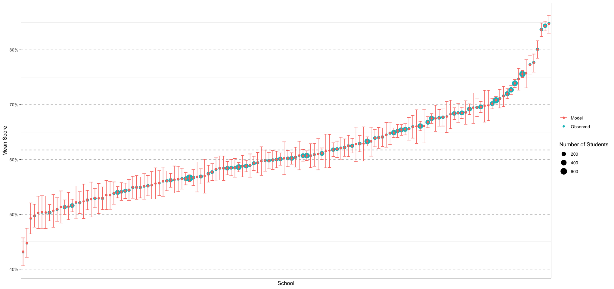
Great! So again we’re doing a good job of capturing the data. This data is very similar to the unpooled estimate, probably because there’s not a lot of variation explained by the different schools. Now let’s pool all of the schools by district!
alberta_schools_authority_pooled_code <- "
data {
    int<lower = 0> N_schools;
    int<lower = 0> N_authorities;
    array[N_schools] real<lower = 0, upper = 1> school_mean;
    array[N_schools] int<lower = 0> school_n;
    array[N_schools] int<lower = 1, upper = N_authorities> authority_index;
}
parameters {
    array[N_schools] real<lower = 0, upper = 1> school_mu;
    array[N_schools] real<lower = 0> school_nu_raw;

    real<lower = 0> authority_prior_alpha_mean;
    real<lower = 0> authority_prior_alpha_sd;
    array[N_authorities] real<lower = 0> school_prior_alpha_raw;

    real<lower = 0> authority_prior_beta_mean;
    real<lower = 0> authority_prior_beta_sd;
    array[N_authorities] real<lower = 0> school_prior_beta_raw;

    real <lower = 0> school_prior_nu_mean;
    real <lower = 0> school_prior_nu_sd;
}
transformed parameters {
    array[N_schools] real<lower = 0> school_alpha;
    array[N_schools] real<lower = 0> school_beta;
    array[N_schools] real<lower = 0> school_sigma_squared;
    array[N_schools] real<lower = 0> school_nu;
    array[N_authorities] real<lower = 0> school_prior_alpha;
    array[N_authorities] real<lower = 0> school_prior_beta;

    for (i in 1:N_authorities) {
        school_prior_alpha[i] = authority_prior_beta_mean + authority_prior_beta_sd * school_prior_beta_raw[i];
        school_prior_beta[i] = authority_prior_alpha_mean + authority_prior_alpha_sd * school_prior_alpha_raw[i];
    }
    for (i in 1:N_schools) {
        school_nu[i] = school_prior_nu_mean + school_prior_nu_sd * school_nu_raw[i];
        school_alpha[i] = school_mu[i] * school_nu[i];
        school_beta[i] = (1 - school_mu[i]) * school_nu[i];
        school_sigma_squared[i] = (school_alpha[i] * school_beta[i]) / (( school_alpha[i] + school_beta[i])^2 * (school_alpha[i] + school_beta[i] + 1));
    }
}
model {
    for (i in 1:N_schools) {
        school_mu[i] ~ beta(school_prior_alpha[authority_index[i]], school_prior_beta[authority_index[i]]);
        school_mean[i] ~ normal(school_mu[i], sqrt(school_sigma_squared[i] / school_n[i]));
    }
    school_nu_raw ~ std_normal(); // non-centred - implies school_nu ~ normal(school_prior_nu_mean, school_prior_nu_sd)

    // TODO create a shared prior for the hyperparameters alpha and beta
    authority_prior_alpha_mean ~ normal(3, 0.5);
    authority_prior_alpha_sd ~ exponential(1);
    authority_prior_beta_mean ~ normal(1, 0.3);
    authority_prior_beta_sd ~ exponential(1);

    school_prior_alpha_raw ~ std_normal();
    school_prior_beta_raw ~ std_normal();

    school_prior_nu_mean ~ normal(30, 4);
    school_prior_nu_sd ~ exponential(1);
}
"
alberta_schools_authority_fit <- run_schools_model(alberta_schools_authority_pooled_code)
alberta_schools_authority_fit$summary()
Running MCMC with 4 sequential chains...
All 4 chains finished successfully.
Mean chain execution time: 14.9 seconds.
Total execution time: 60.0 seconds.| variable | mean | median | sd | mad | q5 | q95 | rhat | ess_bulk | ess_tail |
|---|---|---|---|---|---|---|---|---|---|
| <chr> | <dbl> | <dbl> | <dbl> | <dbl> | <dbl> | <dbl> | <dbl> | <dbl> | <dbl> |
| lp__ | 242.7581233 | 243.4775000 | 20.319465354 | 19.953572100 | 208.5067000 | 275.4238000 | 1.0037834 | 866.746 | 1539.503 |
| school_mu[1] | 0.6387844 | 0.6387405 | 0.007867415 | 0.007838506 | 0.6258293 | 0.6516180 | 1.0017875 | 7730.782 | 3023.918 |
| school_mu[2] | 0.8468010 | 0.8471110 | 0.008234859 | 0.008496039 | 0.8331503 | 0.8597739 | 1.0019272 | 8346.506 | 2944.039 |
| school_mu[3] | 0.6178737 | 0.6180900 | 0.006078236 | 0.006126845 | 0.6077802 | 0.6278174 | 1.0005921 | 7897.363 | 3082.192 |
| school_mu[4] | 0.6220775 | 0.6221365 | 0.008252685 | 0.008003816 | 0.6084058 | 0.6355993 | 1.0035225 | 9066.323 | 2903.928 |
| school_mu[5] | 0.6089325 | 0.6090580 | 0.010396388 | 0.010213631 | 0.5917600 | 0.6258283 | 1.0004491 | 8822.524 | 2701.826 |
| school_mu[6] | 0.5651614 | 0.5651690 | 0.012056050 | 0.012080966 | 0.5459932 | 0.5843686 | 1.0016742 | 8920.377 | 2358.078 |
| school_mu[7] | 0.7564602 | 0.7566715 | 0.013304278 | 0.013247031 | 0.7337154 | 0.7776436 | 1.0003112 | 8465.891 | 2869.356 |
| school_mu[8] | 0.6607885 | 0.6612545 | 0.015222589 | 0.015111400 | 0.6355575 | 0.6852125 | 1.0003871 | 7745.071 | 3102.663 |
| school_mu[9] | 0.5033227 | 0.5035615 | 0.014959102 | 0.014415320 | 0.4786364 | 0.5275542 | 1.0018842 | 7362.804 | 2435.936 |
| school_mu[10] | 0.5489648 | 0.5489295 | 0.009962331 | 0.010085386 | 0.5327384 | 0.5654756 | 1.0009309 | 7858.609 | 2480.194 |
| school_mu[11] | 0.6069848 | 0.6070440 | 0.013525705 | 0.012806699 | 0.5846459 | 0.6296254 | 1.0003953 | 7109.660 | 2533.558 |
| school_mu[12] | 0.6785647 | 0.6788500 | 0.014326434 | 0.014209238 | 0.6543459 | 0.7016713 | 1.0013475 | 8032.309 | 2550.878 |
| school_mu[13] | 0.7764559 | 0.7766735 | 0.008665420 | 0.008676916 | 0.7621878 | 0.7902724 | 1.0022818 | 8470.686 | 2569.698 |
| school_mu[14] | 0.5940918 | 0.5941210 | 0.009433348 | 0.009140970 | 0.5780491 | 0.6095894 | 0.9994629 | 7222.579 | 2868.847 |
| school_mu[15] | 0.5822622 | 0.5822365 | 0.010469228 | 0.010771089 | 0.5654695 | 0.5993273 | 1.0011668 | 8890.172 | 2870.622 |
| school_mu[16] | 0.5611338 | 0.5611185 | 0.008928162 | 0.008979367 | 0.5461858 | 0.5759718 | 0.9999743 | 8275.079 | 2942.549 |
| school_mu[17] | 0.6552331 | 0.6551580 | 0.010271325 | 0.010408593 | 0.6387280 | 0.6719518 | 1.0008111 | 8512.814 | 2635.261 |
| school_mu[18] | 0.7017329 | 0.7018120 | 0.005121847 | 0.005091248 | 0.6931912 | 0.7099870 | 1.0011110 | 7544.982 | 2962.647 |
| school_mu[19] | 0.5692686 | 0.5692310 | 0.007138546 | 0.007034937 | 0.5576670 | 0.5809718 | 1.0041092 | 6968.875 | 2653.758 |
| school_mu[20] | 0.6290081 | 0.6291435 | 0.007791504 | 0.007737689 | 0.6161220 | 0.6418232 | 1.0018235 | 7827.995 | 2969.588 |
| school_mu[21] | 0.5297266 | 0.5297355 | 0.009124199 | 0.009122438 | 0.5144827 | 0.5445661 | 1.0005499 | 7307.825 | 2901.814 |
| school_mu[22] | 0.6477019 | 0.6477230 | 0.010225237 | 0.010181756 | 0.6304554 | 0.6646334 | 1.0012374 | 7897.992 | 2363.115 |
| school_mu[23] | 0.5891082 | 0.5892005 | 0.010622697 | 0.010529425 | 0.5712892 | 0.6062800 | 1.0007224 | 7841.715 | 2924.020 |
| school_mu[24] | 0.5413668 | 0.5413110 | 0.007999754 | 0.007971199 | 0.5283126 | 0.5546806 | 1.0014882 | 8305.301 | 2780.133 |
| school_mu[25] | 0.5880985 | 0.5882500 | 0.010154796 | 0.009871151 | 0.5715252 | 0.6044875 | 1.0009068 | 7350.320 | 2446.588 |
| school_mu[26] | 0.5064102 | 0.5062810 | 0.015608235 | 0.015106953 | 0.4805963 | 0.5324869 | 1.0005418 | 6929.813 | 2712.310 |
| school_mu[27] | 0.6151159 | 0.6152560 | 0.015493198 | 0.015774864 | 0.5897355 | 0.6402394 | 1.0003265 | 7670.134 | 2554.444 |
| school_mu[28] | 0.6982921 | 0.6985970 | 0.014558349 | 0.015005395 | 0.6741918 | 0.7219588 | 1.0000773 | 8525.254 | 3075.386 |
| school_mu[29] | 0.6944085 | 0.6943485 | 0.013937068 | 0.013428649 | 0.6708920 | 0.7171905 | 1.0034761 | 9790.319 | 2710.654 |
| ⋮ | ⋮ | ⋮ | ⋮ | ⋮ | ⋮ | ⋮ | ⋮ | ⋮ | ⋮ |
| school_prior_beta[26] | 6.444429 | 5.945595 | 2.176390 | 1.812382 | 3.942815 | 10.682965 | 1.000358 | 2368.802 | 2829.265 |
| school_prior_beta[27] | 6.228340 | 5.690555 | 2.115253 | 1.673648 | 3.876286 | 10.295395 | 1.000566 | 2573.989 | 2812.977 |
| school_prior_beta[28] | 6.564124 | 6.159870 | 2.046347 | 1.858002 | 4.032383 | 10.587910 | 1.002567 | 1435.181 | 1861.186 |
| school_prior_beta[29] | 6.679653 | 6.131620 | 2.304941 | 1.909085 | 4.031681 | 11.070340 | 1.001554 | 2155.847 | 2806.314 |
| school_prior_beta[30] | 6.215432 | 5.779615 | 1.949213 | 1.717718 | 3.897775 | 9.921474 | 1.000991 | 2442.833 | 2637.715 |
| school_prior_beta[31] | 6.405481 | 5.840280 | 2.213723 | 1.831693 | 3.904279 | 10.745250 | 1.002140 | 2487.839 | 2745.415 |
| school_prior_beta[32] | 6.358579 | 5.781295 | 2.259589 | 1.772270 | 3.870992 | 10.748180 | 1.000821 | 2536.184 | 2771.503 |
| school_prior_beta[33] | 6.104454 | 5.684775 | 1.897604 | 1.599785 | 3.863385 | 9.878326 | 1.000618 | 2249.636 | 2085.735 |
| school_prior_beta[34] | 7.458583 | 7.225070 | 2.004222 | 1.917728 | 4.653268 | 11.136860 | 1.003457 | 1731.328 | 1917.717 |
| school_prior_beta[35] | 6.945114 | 6.741595 | 1.839731 | 1.845919 | 4.452932 | 10.384055 | 1.000970 | 1898.579 | 2357.969 |
| school_prior_beta[36] | 6.902518 | 6.354700 | 2.391516 | 2.096960 | 4.101835 | 11.606285 | 1.002352 | 1846.991 | 2092.054 |
| school_prior_beta[37] | 6.405285 | 5.885545 | 2.142651 | 1.836156 | 3.931134 | 10.559210 | 1.001356 | 2221.362 | 2639.116 |
| school_prior_beta[38] | 5.961819 | 5.485965 | 1.881591 | 1.508886 | 3.827024 | 9.690220 | 1.001043 | 2653.897 | 2563.266 |
| school_prior_beta[39] | 6.511898 | 6.020150 | 2.161627 | 1.885289 | 3.964761 | 10.635820 | 1.001996 | 1721.177 | 2229.240 |
| school_prior_beta[40] | 6.412868 | 5.955380 | 2.122335 | 1.871167 | 3.949675 | 10.369350 | 1.000598 | 2339.874 | 2541.280 |
| school_prior_beta[41] | 6.277202 | 5.778590 | 2.065970 | 1.698911 | 3.910159 | 10.228230 | 1.001257 | 2913.960 | 2810.728 |
| school_prior_beta[42] | 7.714267 | 7.296960 | 2.467924 | 2.333805 | 4.517787 | 12.305235 | 1.002625 | 1542.396 | 1778.872 |
| school_prior_beta[43] | 6.491070 | 6.000300 | 2.182913 | 1.873065 | 3.941435 | 10.762400 | 1.001407 | 1999.256 | 2222.189 |
| school_prior_beta[44] | 6.169196 | 5.666335 | 2.053389 | 1.671631 | 3.866603 | 10.055040 | 1.000085 | 2892.004 | 2505.539 |
| school_prior_beta[45] | 6.446915 | 5.880865 | 2.254919 | 1.863843 | 3.879132 | 10.766230 | 1.000337 | 2587.126 | 2728.151 |
| school_prior_beta[46] | 6.232384 | 5.723025 | 2.047502 | 1.684271 | 3.902608 | 10.333235 | 1.001648 | 2626.035 | 3080.817 |
| school_prior_beta[47] | 5.964638 | 5.512750 | 1.883736 | 1.532445 | 3.801014 | 9.786658 | 1.000639 | 3195.178 | 2958.786 |
| school_prior_beta[48] | 6.243338 | 5.748345 | 2.088923 | 1.725405 | 3.836314 | 10.384930 | 1.001729 | 1967.245 | 2267.657 |
| school_prior_beta[49] | 6.452798 | 5.940115 | 2.247994 | 1.836385 | 3.953984 | 10.753980 | 1.001421 | 2044.521 | 2594.231 |
| school_prior_beta[50] | 6.408177 | 5.942285 | 2.159334 | 1.873065 | 3.922172 | 10.577890 | 1.002382 | 1653.991 | 2504.470 |
| school_prior_beta[51] | 6.361528 | 5.835470 | 2.142953 | 1.770892 | 3.926255 | 10.548125 | 1.003125 | 2515.924 | 2882.958 |
| school_prior_beta[52] | 5.537106 | 5.180855 | 1.563088 | 1.253642 | 3.698441 | 8.543566 | 1.000231 | 3139.606 | 2477.011 |
| school_prior_beta[53] | 5.809495 | 5.407495 | 1.759563 | 1.462993 | 3.788838 | 9.244379 | 1.000570 | 2770.758 | 2997.078 |
| school_prior_beta[54] | 5.381683 | 5.021960 | 1.492077 | 1.180565 | 3.664767 | 8.278310 | 1.000186 | 3755.497 | 2987.081 |
| school_prior_beta[55] | 6.031982 | 5.552770 | 1.968935 | 1.581526 | 3.816465 | 9.846426 | 1.001208 | 2709.514 | 2989.905 |
authority_pooled_school_means_plot <- generate_school_plot(alberta_schools_authority_fit)
print(authority_pooled_school_means_plot)
Again, it looks like this is working basically as expected!
Final Comments
And there we have it! Solving the same problem with various levels of pooling.
One thing that you probably noticed is that all of the results for the last problem were essentially identical! That is absolutely the case, and is perhaps an illustrative example of why you should test out examples before applying these methods. But why did the level of pooling we did seem to have so little effect? Essentially, we had too much data! Pooling works by affecting the prior, and since all of our schools had a large number of students, their data overwhelmed the prior, regardless of whether that prior was unique to the school, pooled among all of the schools, or pooled by authority. As a result, we didn’t see the same changes that we did in the earlier examples, where had had fewer data points. This is unsurprising in retrospect, but it also highlights that pooling has the greatest effect when you do not have an abundance of data.
You might also have noticed that the shape of the models changed as we added levels. That is because I had to reparameterize the models from centred to a non-centred for several parameters in order to avoid issues with the sampler (divergent transitions, &c.). I didn’t go into details here because the focus was on other parts of the process, but I wrote all of the pooled models several times, non-centring a single parameter, then running it to see if it fixed the process, and repeating until everything worked. Apparently it’s very common to have to do this with hierarchical models!
Hopefully this helps with understanding how to build hierarchical models! This is definitely something that I need to work through every time, starting from the unpooled version and then gradually adding in pooling. Despite the added level of complexity, the additional out-of-sampling accuracy and the additional confidence that that engenders in the model is worth it!
sessionInfo()R version 4.4.1 (2024-06-14)
Platform: aarch64-apple-darwin23.4.0
Running under: macOS 15.0.1
Matrix products: default
BLAS: /opt/homebrew/Cellar/openblas/0.3.28/lib/libopenblasp-r0.3.28.dylib
LAPACK: /opt/homebrew/Cellar/r/4.4.1/lib/R/lib/libRlapack.dylib; LAPACK version 3.12.0
locale:
[1] en_CA/en_CA/en_CA/C/en_CA/en_CA
time zone: America/Edmonton
tzcode source: internal
attached base packages:
[1] stats graphics grDevices utils datasets methods base
other attached packages:
[1] readxl_1.4.3 posterior_1.6.0 cmdstanr_0.8.1 ggplot2_3.5.1