Confidence Intervals for the Difference of Means (Small Sample Sizes)
This blog post discusses how to calculate confidence intervals for the difference of means when dealing with small sample sizes, specifically addressing cases where the variances of the two populations are either equal or unequal. The post concludes by demonstrating the application of these methods to paired observations.
Confidence Intervals for the Difference of the Mean - Small Sample Sizes
Previously, I took a look at finding the confidence intervals for the difference of two means, but I assumed that the sample size was large. This greatly simplified the process by allowing us to assume that the distribution of the differences was therefore normally distributed. However, we often deal with cases where we have a small sample, and so cannot use this approximation. In this post, I’ll go through how we can establish a confidence interval for the mean even when the sample size is small.
small and
The first case that we’ll look at is where the number of samples is small and we have reason to believe that the variances of the two populations are the same. In the case of a large sample, we would use the following fact to derive our confidence interval:
When , then this simplifies to
However, one issue is that we don’t want that there. Since we don’t know what it is, we would prefer to have some expression involving , the sample standard deviation. Thinking back to the previous post, we can play the same trick as we did when deriving the fact that the sampling distribution for means with small was the distribution (because in fact, we’re doing the same thing).
We know that and . In addition, we know that if and , then . Combining these,
Again using the same trick as earlier, we know that if and , then
Now we just need one more piece of information to come up with a sampling distribution for the mean. Since we believe that there is a common standard deviation, we would like to estimate it from the samples as a whole, rather than using one from the first sample and one from the second. To pool these, we use the formula
Now let’s put it all together!
We can write a new quantity
And thus, if we want a confidence interval, we know that
which then means that the confidence interval for the difference of means is
where is the value for the distribution with degrees of freedom which has area to the right.
Example
In the article Macroinvertebrate community structure as an indicator of acid mine pollution, the authors attempt to determine the relationship between certain physical / chemical parameters and different measures of community diversity among the invertebrates in a creek. Essentially, they wanted to see if they could find a connection between the diversity of the invertebrate community and the level of stress that the community was under (e.g. due to pollution).
They used two different sampling stations: one above the mine discharge and one below. For the downstream site, they collected data once a month for 12 months and found a species diversity with a mean of and standard deviation , while at the upstream site they collected for 10 months and found and . What is the 90% CI for the difference in the means of these two sites, assuming equal variances?
(This is based on example 7.7, p. 228 in Walpole & Myers, 1985)
# data
n_1 <- 12
x_1_bar <- 3.11
s_1 <- 0.771

n_2 <- 10
x_2_bar <- 2.04
s_2 <- 0.448

# confidence level
alpha <- 0.1

# calculated values
diff <- x_1_bar - x_2_bar # 1.07
s_p <- sqrt(((n_1 - 1)*s_1^2 + (n_2 - 1)*s_2^2) / (n_1 + n_2 - 2)) # 0.646
df <- n_1 + n_2 - 2 # degrees of freedom for the t distribution
t_alpha_2 <- qt(alpha / 2, df, lower.tail=FALSE) # 1.7247
ci <- diff + c(-1, 1) * t_alpha_2 * s_p * sqrt(1 / n_1 + 1 / n_2)
ci- 0.592974151120243
- 1.54702584887976
This tells us that we are 90% confident that the index for the downstream observations are higher than for the upstream ones (0.59 - 1.55 higher). Just as before, we can also examine this graphically.
library(ggplot2)

add_annotated_arrow <- function(p, start, end, text=NA, text_shift=c(0,0)) {
    p <- p +
    geom_segment(aes(x=start[1], y=start[2], xend=end[1], yend=end[2]), arrow=arrow())

    if (!is.na(text)) {
        p <- p + annotate('text', x=start[1] + text_shift[1], y=start[2] + text_shift[2], label=text)
    }
    return(p)
}

x <- seq(-3, 3, by=0.01)
plot_df <- data.frame(x=x, y=dt(x, df))

p <- ggplot(plot_df, aes(x, y)) +
    geom_line(linewidth=2) +
    # area
    geom_ribbon(data=subset(plot_df, x >= -t_alpha_2 & x <= t_alpha_2), aes(ymax=y), ymin=0, fill="blue", alpha=0.5) +
    # critical points
    geom_segment(aes(x=-t_alpha_2, y=0, xend=-t_alpha_2, yend=dt(-t_alpha_2, df)), linewidth=2) +
    geom_segment(aes(x=t_alpha_2, y=0, xend=t_alpha_2, yend=dt(t_alpha_2, df)), linewidth=2) +
    labs(x='Standardized Difference of Means', y="Density", title="Distribtion of the Standardized Difference of Means")

# add in arrows and annotations
p <- add_annotated_arrow(p, c(2, 0.25), c(t_alpha_2, dt(t_alpha_2, df) + 0.01), text="Critical Points", text_shift=c(0, 0.01))
p <- add_annotated_arrow(p, c(2, 0.25), c(-t_alpha_2, dt(-t_alpha_2, df) + 0.01))
p <- add_annotated_arrow(p, c(-2, 0.3), c(0, 0.25), text="90% Area", text_shift=c(0, 0.01))
print(p)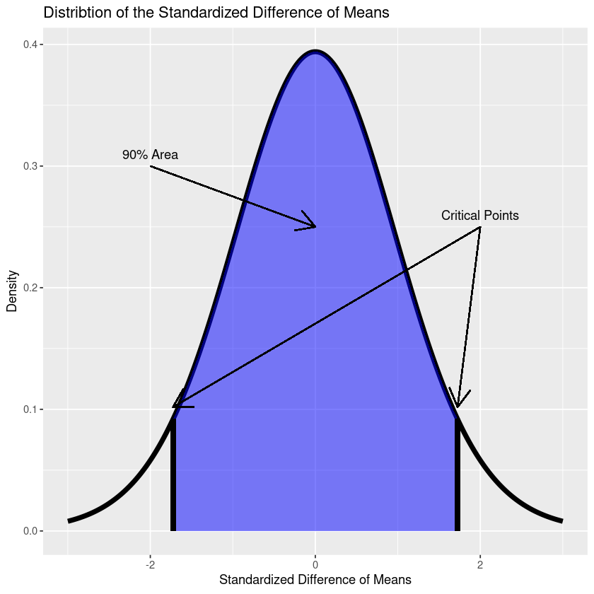
One thing to note is that the above is the distribution for the standardized difference in the means - that is, . To get the confidence interval above we had to perform some manipulations to isolate , which is why we don’t see the distribution centred at the sample difference of means.
and Both Unknown
In the case where we assume that the standard deviations are different, the calculations become immediately far more complex. As a result, many of the results in this section will need to be accepted without a good explanation!
For this case, we generally use the statistics
which is more or less distributed as a distribution with
degrees of freedom (rounded to the nearest integer).
Like I said: this case is much more complex!
If we take that as given, then we can come up with the confidence interval by rearranging for , just as we did before. That gives us the following confidence interval.
Example
Let’s revisit the earlier example on macroinvertebrate community structure, but this time let’s not assume that the variances are the same.
# data
n_1 <- 12
x_1_bar <- 3.11
s_1 <- 0.771

n_2 <- 10
x_2_bar <- 2.04
s_2 <- 0.448

# confidence level
alpha <- 0.1

# calculated values
diff <- x_1_bar - x_2_bar # 1.07 - same as before
# degrees of freedom for the t distribution - was 20, now 18
df <- round((s_1^2 / n_1 + s_2^2 / n_2)^2 / ((s_1^2 / n_1)^2 / (n_1 - 1) + (s_2^2 / n_2)^2 / (n_2 - 1)))
t_alpha_2 <- qt(alpha / 2, df, lower.tail=FALSE) # 1.7247 -> 1.73
different_variances_ci <- diff + c(-1, 1) * t_alpha_2 * sqrt(s_1^2 / n_1 + s_2^2 / n_2)
different_variances_ci- 0.612499103092034
- 1.52750089690797
Recall that the old confidence interval was (0.59 - 1.55); by not assuming that the variances are equal we’ve slightly shrunk the interval.
plot_df <- data.frame(
    category=c("Equal variances", "Different Variances"),
    lower=c(ci[1], different_variances_ci[1]),
    upper=c(ci[2], different_variances_ci[2]),
    centre=c(mean(ci), mean(different_variances_ci))
)

p <- ggplot(plot_df, aes(x=category)) +
    geom_linerange(aes(ymin=lower, ymax=upper)) +
    geom_point(aes(y=centre)) +
    labs(title="Comparing 90% Confidence Intervals - Assuming Equal Variances and Not", x="Category", y="Difference in Means")

print(p)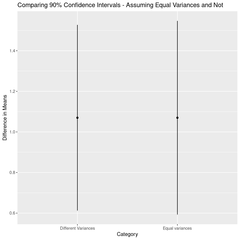
Seeing the graph makes it clear that the intervals are very close.
Paired Observations
Just to close off, let’s take a look at a case that we have secretly already solved: the case where we have two sets of observations, but now the samples are dependent. This could occur in the case where we measure something of interest, make some change, then measure it again on the same group of subject. For instance, maybe you’re testing the effect of exercise on weight loss. In that case, you might weigh a group of subject, have them exercise for a month, then measure their weights again to see what happened. Since you are measuring the same subjects, the two samples are no longer independent, and as such, the prodcedures that we have used so far would be inappropriate.
Or are they?
In fact, we can use our existing techniques if we focus not on the before and after measurements, but instead on their differences. Those differences should be independent, and so really now we are looking for a single-sample confidence interval for the mean; something we already know how to do!
If the true difference in means is and the sample difference in means is , and assuming that we’re dealing with a smallish sample size (and so are using instead of ), then the quantity
has a distribution with degrees of freedom, and so the confidence interval for the difference in means is
Example
(The following is based on example 7.9 in Walpole and Myers (1985), p. 232).
In “Essential Elements in Fresh and Canned Tomatoes”, the authors looked at the essential elements found in tomatoes both before and after canning. The results for copper are as follows:
| Fresh | Canned |
|---|---|
| 0.066 | 0.085 |
| 0.079 | 0.088 |
| 0.069 | 0.091 |
| 0.076 | 0.096 |
| 0.071 | 0.093 |
| 0.087 | 0.095 |
| 0.071 | 0.079 |
| 0.073 | 0.078 |
| 0.067 | 0.065 |
| 0.062 | 0.068 |
Find a 98% confidence interval for the true difference in mean copper content between fresh and canned tomatoes, assuming the distribution of differences to be normal.
First, let’s visualize what these differences look like.
tomatoes <- data.frame(
    fresh=c(
        0.066,
        0.079,
        0.069,
        0.076,
        0.071,
        0.087,
        0.071,
        0.073,
        0.067,
        0.062
    ),
    canned=c(
        0.085,
        0.088,
        0.091,
        0.096,
        0.093,
        0.095,
        0.079,
        0.078,
        0.065,
        0.068
    )
)

ggplot(tomatoes, aes(y=1:nrow(tomatoes))) +
    geom_point(aes(x=fresh, colour='Fresh')) +
    geom_point(aes(x=canned, colour='Canned')) +
    geom_linerange(aes(xmin=fresh, xmax=canned, colour=ifelse(canned - fresh > 0, "Increase", "Decrease"))) +
    labs(title="Before-and-After Comparisons of Copper Content in Tomatoes", x="Copper Content", y="Sample") +
    theme(axis.text.y = element_blank(), axis.ticks.y = element_blank())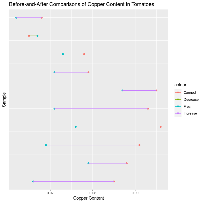
As we can see, there is a definite correlation between the two samples: tomatoes with a small copper content before tend to have a small copper content after, and so on. So now instead, let’s look at the differences!
tomatoes$d <- tomatoes$canned - tomatoes$fresh
tomatoes| fresh | canned | d |
|---|---|---|
| <dbl> | <dbl> | <dbl> |
| 0.066 | 0.085 | 0.019 |
| 0.079 | 0.088 | 0.009 |
| 0.069 | 0.091 | 0.022 |
| 0.076 | 0.096 | 0.020 |
| 0.071 | 0.093 | 0.022 |
| 0.087 | 0.095 | 0.008 |
| 0.071 | 0.079 | 0.008 |
| 0.073 | 0.078 | 0.005 |
| 0.067 | 0.065 | -0.002 |
| 0.062 | 0.068 | 0.006 |
alpha = 0.02
n = nrow(tomatoes)
sd <- sd(tomatoes$d) # 0.0084
d_bar <- mean(tomatoes$d) # 0.0117
df <- n - 1 #degrees of freedom
t_alpha_2 <- qt(1 - alpha / 2, n - 1) # 2.81

ci <- d_bar + c(-1, 1) * t_alpha_2 * sd / sqrt(n)
ci- 0.00421092600527412
- 0.0191890739947259
And from there we have that the 98% confidence interval for the difference in copper content between canned and fresh tomatoes is an increase of 0.0042 - 0.0019.
For fun, we can also use the built-in t.test function to get this interval. This function requires the raw data (rather than the samples statistics like ), so we couldn’t use it in the earlier examples.
result <- t.test(tomatoes$d, conf.level=0.98)
result
One Sample t-test
data: tomatoes$d
t = 4.4079, df = 9, p-value = 0.001701
alternative hypothesis: true mean is not equal to 0
98 percent confidence interval:
0.004210926 0.019189074
sample estimates:
mean of x
0.0117Conclusion
So there you have it! We’ve covered methods to derive confidence intervals for the difference of means between two populations in cases where the number of samples, , is small; in particular, too small to be able to assume normality.
Bibliography
- Walpole, R. E., & Myers, R. H. (1985). Probability and Statistics for Engineers and Scientists. Macmillan USA.
- Dills, G., & Rogers, D. T. (1974). Macroinvertebrate community structure as an indicator of acid mine pollution. Environmental Pollution (1970), 6(4), 239–262. https://doi.org/10.1016/0013-9327(74)90013-5
- Essential Elements in Fresh and Canned Tomatoes—LOPEZ - 1981—Journal of Food Science—Wiley Online Library. (n.d.). Retrieved 7 December 2023, from https://ift.onlinelibrary.wiley.com/doi/abs/10.1111/j.1365-2621.1981.tb04878.x